Basic OSPF operations

This is Part 1 of 3 of OSPF (Open Shortest Path First) CCNA study notes. OSPF is the only dynamic routing protocol explicitly named in the CCNA exam topics list. This lesson focuses on basic OSPF operations and configurations. This lesson introduces foundational concepts related to the function, operations, and deployment of OSPF. We learn how to configure OSPF on a router, how to configure a passive interface on a router, how to advertise a default route into OSPF, and how to manually configure a router ID on a router. Specifically, this post covers CCNA topic 3.4 which says you must be able to “Configure and verify single area OSPFv2”; more specifically, this post covers subtopics 3.4a Neighbor adjacencies and 3.4d Router ID. 

OSPF Part 2, How routers become OSPF neighbors, covers the seven OSPF neighbor states, three methods to change the OSPF cost, how to configure OSPF directly on a router interface, and how to configure passive OSPF interfaces.

OSPF Part 3, OSPF network types, covers the role and election of designated and backup designated routers in a subnet, how to configure the OSPF interface priority on a router in an OSPF broadcast network, how to configure the clock rate on the DCE side of a serial connection, how to configure PPP encapsulation on a point-to-point router, how to manually configure the OSPF network type of an interface on a router, OSPF neighbor/adjacency requirements (troubleshooting adjacency problems), and the role of Type 1, Type 2 and Type 3 LSAs in IP connectivity within OSPF areas.

The lesson on dynamic routing introduced dynamic routing protocols types, algorithms, and metrics. You may want to review it before diving into this lesson. It covered some important background information that situates OSPF within the broader context of routing protocols in terms of general characteristics and functionality. There is also a continuity between this lesson, Basic OSPF operations, and the lesson on RIP & EIGRP configuration and function. This post constitutes Issue 21 of my CCNA 200-301 study notes.

• Background for OSPF
• Basic OSPF operations – introduction
• LSA flooding
• OSPF areas
• OSPF areas – a few additional rules
• Basic OSPF configuration
• passive-interface command
• Advertise a default route into OSPF
• show ip protocols
• Command review
• Key learnings
• Practice quiz questions
• Key references

You may also be interested in CCNA 200-301 study notes.

Background for OSPF

Dynamic routing can be contrasted with static routing. Static routing involves manually configuring routes to each destination. In large networks it is not practical to use only static routes, you would have to configure thousands of different routes, which can become unwieldy. In comparison, dynamic routing involves configuring a dynamic routing protocol on a router and then letting the router take care of finding the best routes to destination networks.

Dynamic routing protocols allow routers to automatically learn routes to different destinations without having to manually configure routes. If multiple routes to a destination are learned, the router determines which route is superior and adds it to the routing table. Routers use the metric of the route to decide which route is superior, and the lower metric is superior.

The term “dynamic” is used because the routing tables are updated dynamically as the network conditions change. If one path to a destination becomes unavailable, the routers will automatically start using the next best path, and the routing tables will be updated to reflect the change.

Most large networks use dynamic routing because it provides a more efficient and reliable way to route traffic than static routing. Dynamic routing is also used in smaller networks where the network conditions are constantly changing.

Here are some of the benefits of using dynamic routing:

• Better performance: Dynamic routing can help to improve network performance by routing traffic around congested links.
• Increased reliability: Dynamic routing can help to increase network reliability by routing traffic around failed links.
• Easier scalability: Dynamic routing can make it easier to scale networks by automatically adding new routes as the network grows.

Here are some of the drawbacks of using dynamic routing:

• Complexity: Dynamic routing can be more complex to configure and manage than static routing.
• Resource consumption: Dynamic routing can consume more resources, such as CPU and memory, than static routing.
• Security risks: Dynamic routing can introduce security risks, such as routing loops and denial-of-service attacks.

Basic OSPF operations – introduction

Recall, RIP and EIGRP are both distance vector routing protocols belonging to the IGP (Interior Gateway Protocol) category of dynamic routing protocols. OSPF and IS-IS are both link state routing protocols also of the IGP type.

Let’s quickly review how link state routing protocols function.

• When using a link state routing protocol, every router creates a connectivity map of the network.
• To allow this, each router advertises information about its interfaces (its connected networks) to its neighbors. These advertisements are passed along to other routers until all routers in the network develop the same complete map of the network.
• Then, each router independently uses this map to calculate the best routes to each destination.
• Link state protocols require more CPU resources on the router than distance vector protocols because they share more information.
• However, link state protocols tend to be faster in reacting to changes in the network than distance vector protocols. 

This lesson focuses only on OSPF, specifically, OSPFv2. There are three versions of OSPF.

• OSPFv1 was released in 1989. It’s old and no longer in use.
• OSPFv2 was released in 1998. This is typically the version that is used in IPv4 networks. OSPFv2 only supports IPv4.
• OSPFv3 was developed for IPv6. It can also be used for IPv4, but OSPFv2 is more common in IPv4 networks. OSPFv3 is a more scalable and efficient protocol than OSPFv2, and it offers a number of new features, such as authentication and encryption.

The version of OSPF specified in the CCNA exam topics list is version 2. When we talk about OSPF in this document, we are talking about version 2. 

Routers configured with dynamic routing protocols such as OSPF, EIGRP, and RIP form adjacencies, also known as neighbor relationships or neighborships, with adjacent routers to exchange routing information.

OSPF routers use LSAs (Link-State Advertisements) to update neighboring routers about a router’s interfaces. LSAs include the following information: the router’s ID, the interface’s IP address, the interface’s subnet mask, and the interface’s cost. LSAs are organized in a structure called the LSDB (Link State Database).

OSPF routers will flood LSAs until all routers in the OSPF area develop the same view of the network. OSPF routers in adjacencies share a common map, an LSDB, that covers an OSPF area.

Note: the process of how routers become OSPF neighbors and start exchanging routing information is better explained in OSPF Part 2 study notes.

OSPF routers use the “shortest path first” algorithm, created by Dutch computer scientist Edsger Dijkstra, to calculate the shortest paths to all destinations in the network. Another name for the SPF algorithm is Dijkstra’s algorithm.

LSA flooding

The following network of four routers is running OSPF. The routers are OSPF neighbors.

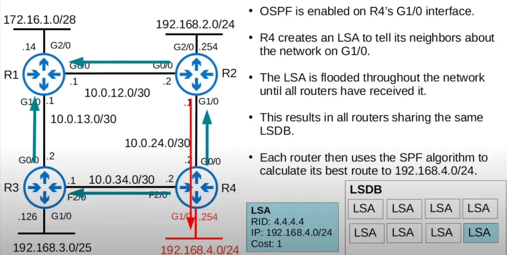
OSPF is enabled on R4’s G1/0 interface. So R4 creates an LSA with the following information to tell its OSPF neighbors about the 192.168.4.0/24 network segment on G1/0:

RID (router ID): 4.4.4.4
IP: 192.168.4.0/24
Cost: 1

The LSA is then flooded throughout the network until all routers receive a copy (follow the green arrows in the above diagram). This results in all routers in the OSPF area having the same LSDB. The LSDB contains LSAs for all the different links in the network. Now that OSPF has been activated on R4’s G1/0 interface, that new LSA is added to the LSDB. 

Note R4’s router ID is 4.4.4.4. None of R4’s physical interfaces have an IP address of 4.4.4.4, so either R4 has a loopback interface with the IP address 4.4.4.4 or the router ID was manually configured. How the router ID is determined (and manually configured) is discussed shortly.

The network 192.168.4.0/24 on R4’s G1/0 interface is included in the LSA. After all, the main purpose of the LSA is to advertise networks connected to OSPF activated interfaces. R4’s cost is also included (OSPF’s metric is called cost). This GigabitEthernet interface has a cost of 1. 

The LSDB is identical for all routers in the OSPF area. Each router then uses the SPF algorithm to calculate its best route to 192.168.4.0/24. Remember, each of these routers has a complete map of the network. R2 would use the map to determine that its (R2’s) best route to 192.168.4.0/24 is via G1/0 (follow the red arrow in the above diagram).

Finally, note that each individual LSA has an aging timer. The LSA is flooded once every 30 minutes by default on Cisco routers.

*In OSPF, there are three main steps in the process of sharing LSAs and determining the best route to each destination in the network. 

Step 1: a router becomes neighbors with other routers connected to the same network segment.

Step 2: exchange LSAs with neighbor routers, as we saw in the above network.

Step 3: each router independently calculates its best routes to each destination, and adds them to the routing table.

These steps are covered in depth in OSPF Part 2 study notes.

OSPF areas 

OSPF areas are a unique aspect of OSPF and a key consideration in network design and management.

*OSPF splits networks into smaller sections called areas.

OSPF areas are identified by a unique area ID, and they can be implemented using subnets, VLANs, physical network segments, or a combination thereof.

*Small networks can be single-area networks without any negative effects on network performance. For example, the previous network with four routers (under the heading LSA flooding) is a small network. 

*In larger networks, however, a single-area design can have some negative effects. For example, if the OSPF network had 500 routers with over 1000 subnets instead of 4 routers and just a few subnets, it would be a bad idea to use just a single OSPF area. 

*Some of the negative effects of using a single-area design in a large network:

• The SPF algorithm takes more time to calculate routes in a large network.
• The SPF algorithm also requires exponentially more processing power on each router to make calculations.
• Each router sharing a large link state database takes up more memory on the routers. 
• Every small change on the network, for example a new interface being activated, would cause every router to flood LSAs to all 500 routers, and all of those routers would have to do the SPF calculation again. 

*Dividing a large OSPF network into several smaller areas helps prevent these negative effects from happening. By dividing a large OSPF network into smaller areas, the number of LSAs that need to be exchanged between routers is reduced. This can lead to decreased routing overhead, faster convergence, and a more stable network.

Here is a brief overview of OSPF areas and how they work. 

This is a larger network than the previous one. 

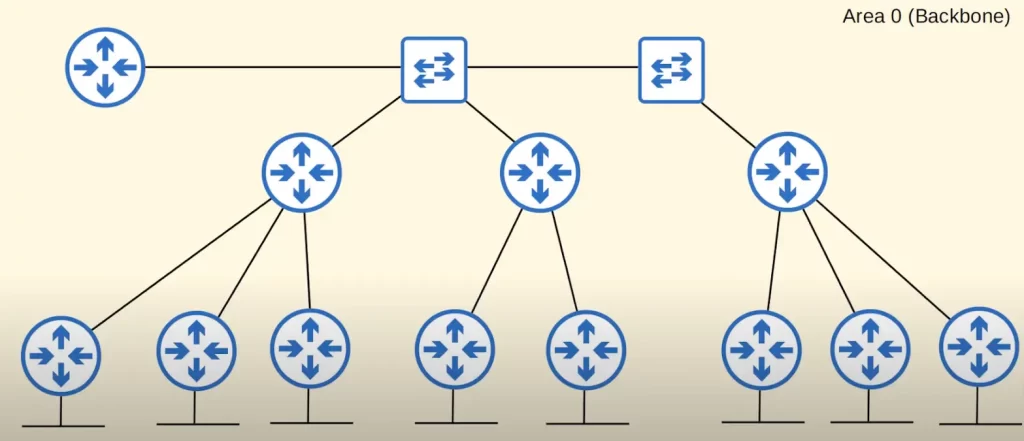
All interfaces on all routers running OSPF are assigned to Area 0, also known as the backbone area. 

Instead of one large area let’s see how the network can be divided into separate areas. 

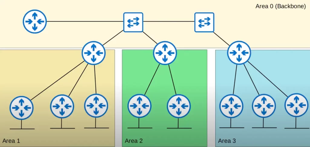
There are some rules and terminology we should know about OSPF areas. 

*An area is a set of routers and links that share the same LSDB. Looking at the above network diagram, there are four areas. Area 0, Area 1, Area 2, and Area 3. Each of these areas maintains a unique LSDB.

*Routers with all interfaces in the same OSPF area are called internal routers. In the above diagram, Area 0 has one internal router, the only router in Area 0. Area 1 has three adjacent internal routers. Area 2 has two adjacent internal routers. And Area 3 has three adjacent internal routers.

*Routers with interfaces in multiple OSPF areas are called area border routers (ABRs) because they are the border between different OSPF areas. In the above network, there are three ABRs – a router connected to Area 0 and Area 1, a router connected to Area 0 and Area 2, and a router connected to Area 0 and Area 3.

It is recommended that you connect an ABR to a maximum of 2 areas. Connecting an ABR to +3 areas can overburden the router, since ABRs maintain a separate LSDB for each area they are connected to.

*In an OSPF network, all areas must connect to the backbone area. The backbone area is a special area that is used to connect all of the other areas in the network. It is also used to exchange routing information between the different areas.

Looking back at the previous network diagram, notice that Area 1, Area 2, and Area 3 all connect to Area 0.

In comparison, the following network design, for example, is not allowed in OSPF. 

Area 1 is not connected to Area 0. Area 1 is only connected to Area 2. This is not allowed in OSPF.

*Routers connected to the backbone area are called backbone routers. This includes ABRs. In the following network the router connected only to Area 0 is a backbone router. It is a backbone router and an internal router, internal to Area 0.

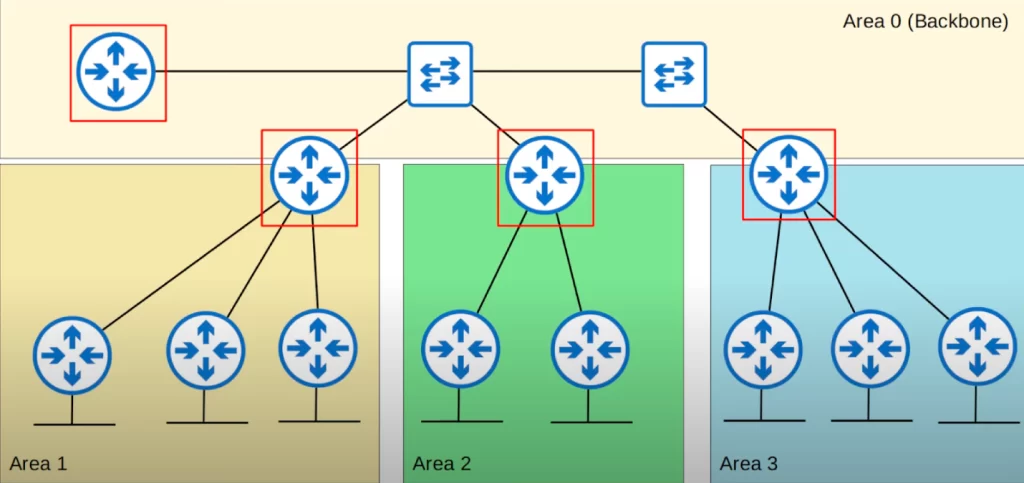
Then there are three routers (in red boxes) that are both backbone routers and ABRs.

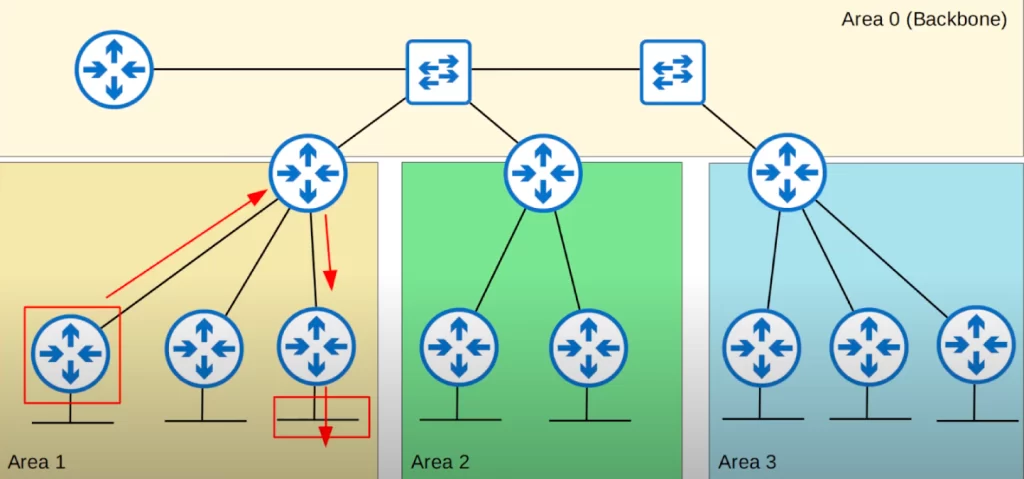
*An intra-area route is a route to a destination inside the same OSPF area. For example, from a router in Area 1 to a destination that is also in Area 1. Let’s see an example. 

If the router in the red box in the below diagram learns a route to the subnet outlined by the red rectangle (follow the red arrows), it is considered an intra-area route, because the destination is in the same area as the router. 

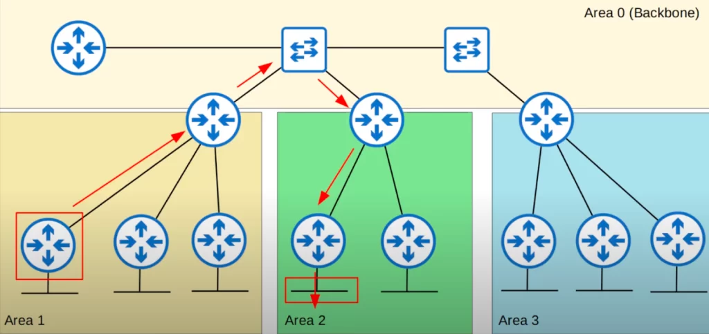
*An inter-area route is a route to a destination in a different OSPF area. For example, if a router in Area 1 learns a route to a destination in Area 2, that is an inter-area route. 

Follow the red arrows in the following diagram: if this router in Area 1 learns a route to this subnet in Area 2, the route is considered an inter-area route. The router and the destination are in two different OSPF areas.

OSPF areas – a few additional rules

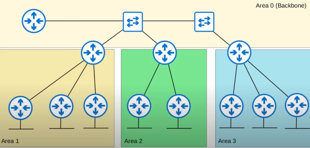
*OSPF areas should be contiguous. Each individual area should be connected, not divided up. The following network satisfies this rule. All areas are contiguous. 

But look now, Area 1 is non-contiguous. Half of Area 1 is on the right side of this network topology, and another half of Area 1 is on the left side of the topology.

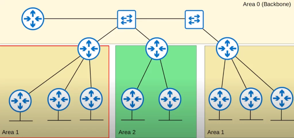
This kind of network design is not allowed in OSPF and will cause problems. We should make the section on the right a separate area, Area 3, so that all the areas become contiguous and OSPF can function properly.

*All OSPF areas must have at least one ABR connected to the backbone area. Let’s look at this network diagram again:

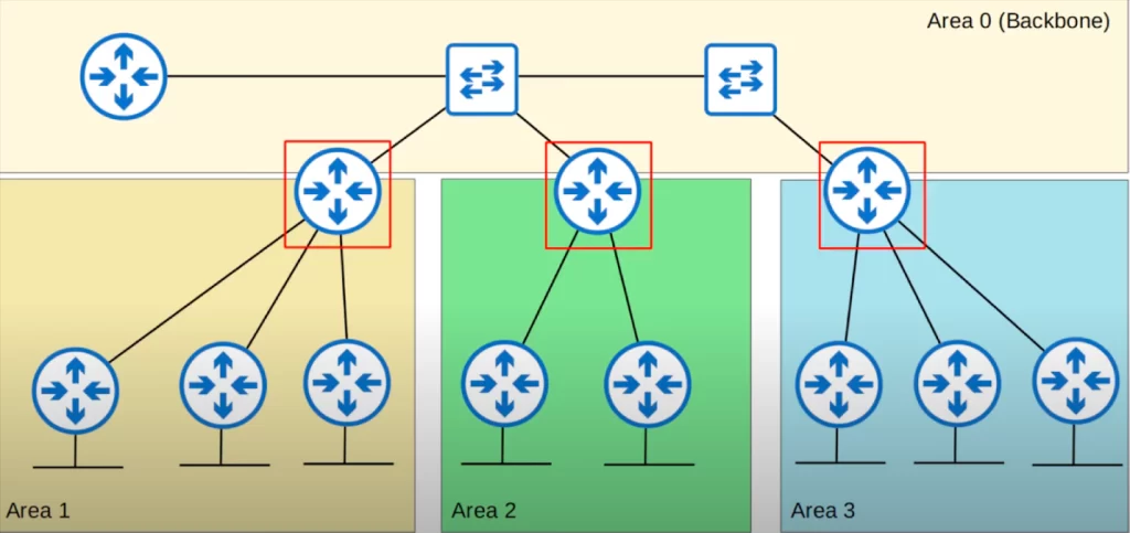
Notice that Area 1 has an ABR connected to both Area 1 and Area 0. Area 2 has an ABR connected to both Area 2 and Area 0. And Area 3 also has an ABR connected to both Area 3 and Area 0. This is correct OSPF network design. 

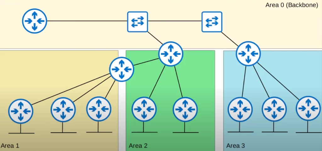
A network like the one below is not correct OSPF design and will cause problems because Area 1 does not have an ABR connected to the backbone area.

*OSPF interfaces in the same subnet must be in the same area. If they are not in the same area, they will not become OSPF neighbors and will not exchange information about the networks they know about. 

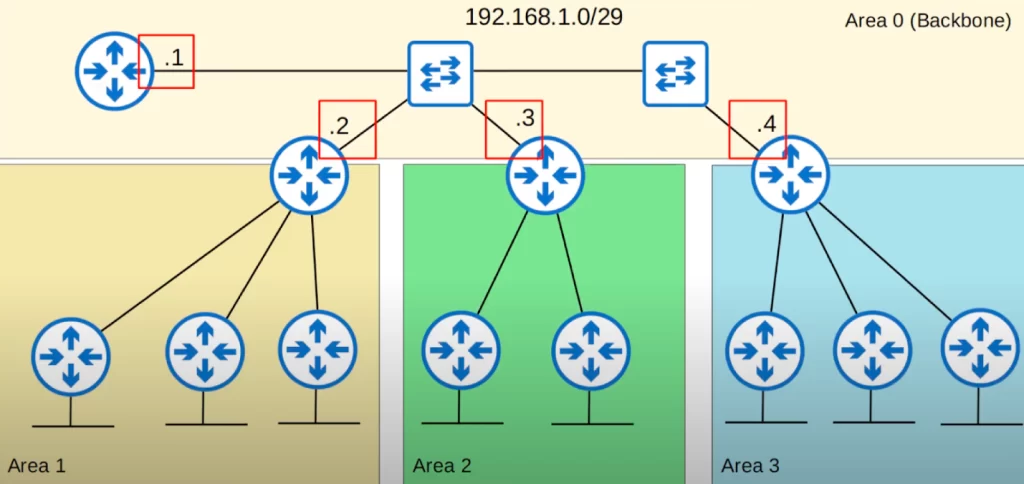
Here is an example to demonstrate this rule. The three routers in red boxes all have an interface in Area 0, in the 192.168.1.0/29 subnet. The router in the green box in Area 1 also has an interface in the 192.168.1.0/29 subnet, but the interface is in Area 1, not Area 0. 

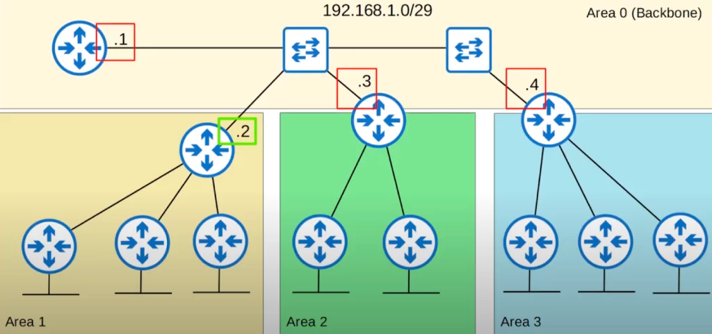
Even though all four interfaces are in the same subnet and OSPF is enabled on them, the Area 1 router will not become OSPF neighbors with the others. 

This time, as shown in the below network, the Area 1 ABR’s interface in the 192.168.1.0/29 subnet is correctly configured in Area 0. So, all four routers will become OSPF neighbors. 

Here’s a summary of those three rules.

• OSPF areas should be contiguous.
• All OSPF areas must have at least one ABR connected to the backbone area.
• OSPF interfaces in the same subnet must be in the same area. 

Basic OSPF configuration

For single area OSPF it is possible to use any area number, but it is considered best practice to use Area 0.

Here is the same network topology we used for RIP and EIGRP. R2, R3, and R4 are already configured. Let’s configure OSPF on R1. All the router interfaces are in OSPF Area 0. 

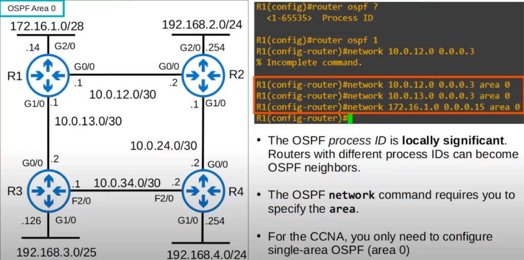
First, from global configuration mode we entered OSPF configuration mode using the command router ospf, followed by a process ID, i.e., 1. 

A router can run multiple OSPF processes at once. The process ID is used in the router to identify each process. The OSPF process ID is locally significant. Routers with different process IDs can become OSPF neighbors.

Next, we attempted to use the network command to configure OSPF on R1, like we did with EIGRP. The router did not accept that command and considered it an “incomplete command”. The OSPF network command requires you to specify the area.

The command syntax for the OSPF network command is as follows.

R(config-router)#network network-address wildcard-mask area area-id

So to activate OSPF on R1’s g0/0 interface with the IP address 10.0.12.1/30, for example, we use the /30 prefix length in the network command. More accurately, we use the wildcard mask equivalent of a /30 subnet mask in the network command.

/30 subnet mask is 255.255.255.252. The wildcard mask equivalent is 0.0.0.3.

R1(config-router)#network 10.0.12.0 0.0.0.3 area 0

We activated OSPF on all the interfaces on R1 in Area 0 using the network command (see the red rectangle in the above CLI output).

When OSPF is activated on the interface, the router will then try to become OSPF neighbors with other OSPF-activated neighbor routers. In this case, R1 will become OSPF neighbors with R2 and R3. 

Here is a quick refresher for how the network command works:

The OSPF NETWORK command tells the router to,

• look for interfaces on the router with an IP address that is in the range specified in the NETWORK command.
• then activate OSPF on the interfaces that fall in the range, in the specified area.
• form adjacencies with other OSPF-activated neighbor routers.
• advertise the networks that are connected to the activated interfaces to the adjacent OSPF routers.

For example, in the first network command we specified 10.0.12.0 with a /30 wildcard mask (0.0.0.3), in Area 0. R1’s G0/0 interface has an IP address of 10.0.12.1, which is contained in 10.0.12.0/30. So OSPF will be activated on G0/0 in Area 0.

Note:

• The configurations covered in this lesson are summarized in the “Key learnings” section.
• Dive deeper: IP Routing: OSPF Configuration Guide (cisco.com)

Next, let’s look at a few other configurations we can do in OSPF. 

passive-interface command

This command was covered in the lesson RIP & EIGRP function and configuration.

The syntax for the passive-interface command is as follows from OSPF configuration mode:

passive-interface [interface | default]

The interface parameter specifies the type and number of the interface. For example, to configure interface FastEthernet0/0 as passive, you would use the following command:

passive-interface FastEthernet0/0

The default keyword can be used to configure all interfaces as passive by default. For example, the following command would configure all interfaces as passive:

passive-interface default

To verify that an interface is configured as passive, you can use the show ip protocols command. The output of this command will show the status of all interfaces, including whether they are configured as passive.

This passive-interface command tells R1 to stop sending OSPF hello messages out of g2/0:

R1(config-router)#passive-interface g2/0

OSPF uses hello messages to tell other routers about itself. Hello messages are sent periodically by OSPF routers to other routers on the network. The hello messages contain information about the router’s ID, the area it belongs to, and the interfaces it is running OSPF on.

Hello messages are used to establish and maintain OSPF neighbor relationships. When two routers receive each other’s hello messages, they know that they are neighbors and can start exchanging routing information. 

OSPF hello messages are sent using IP multicast. The multicast address for OSPF hello messages is 224.0.0.5.

You should always use the passive-interface command on interfaces which do not have any OSPF neighbors. It’s a waste to continuously send hello messages out of an interface with no other routers connected to it.

R1 will continue to send LSAs informing its neighbors about the subnet configured on the g2/0 interface. Although R1 will not send hellos out of g2/0 and try to find OSPF neighbors, it will still tell its OSPF neighbors about the 172.16.1.0/28 network.

OSPF routers advertise the networks of their OSPF interfaces through LSAs, through LSA flooding. LSAs contain the following information about the network: the network address, the subnet mask, and the cost of the network.

OSPF routers will flood LSAs until all routers in the OSPF area develop the same map of the network, meaning the same LSDB. In LSA flooding, each OSPF router floods LSAs to its OSPF neighbors. The LSAs are then flooded to all other OSPF routers in the area until all the routers in the area have the same map of the network. 

LSAs are flooded using multicast addresses to efficiently disseminate routing information within the OSPF network. Multicast addresses used:

• Point-to-point networks: 224.0.0.5
• Broadcast networks: 224.0.0.6

Advertise a default route into OSPF

Next let’s see how to advertise a default route into OSPF, like we did for RIP. First we configure a default route on R1. 

We added an Internet connection to R1 then configured a default route on R1 for the network 0.0.0.0/0, and the next hop is the ISP’s IP address of 203.0.113.2. 

Here is that information in R1’s routing table. Take note of the other OSPF routes that R1 has learned.

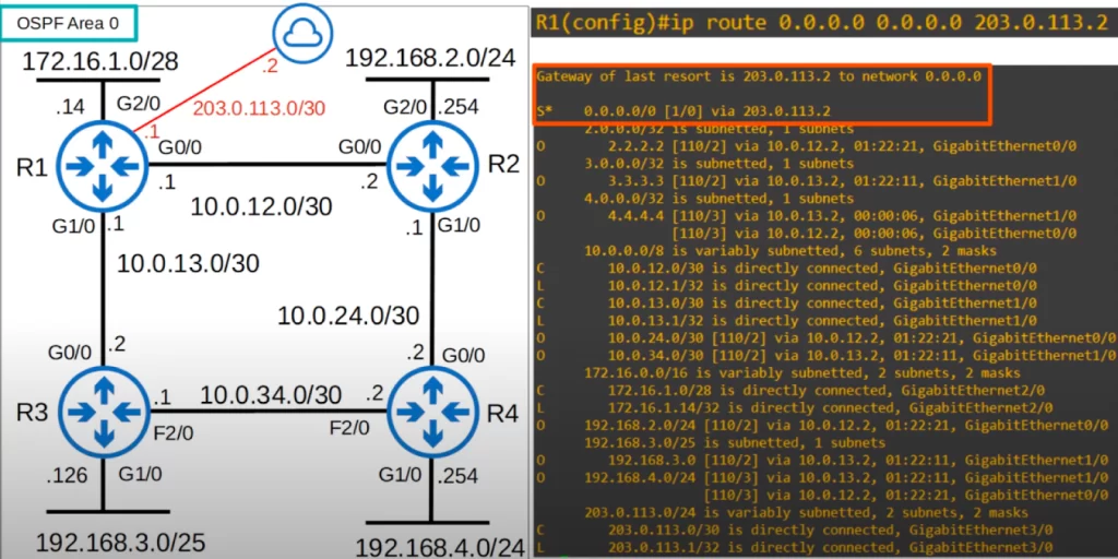
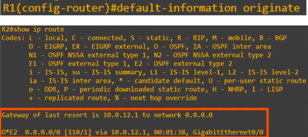
Just like in RIP, the command to advertise the default route into OSPF is default-information originate. In OSPF this will cause the router to create a new LSA and flood it. On checking R2’s routing table, we can see that R2 added the default route via R1 to its routing table. R3 and R4 will each also add an entry for the default route to their routing tables. 

show ip protocols 

Now let’s look at the show ip protocols command from an OSPF perspective. 

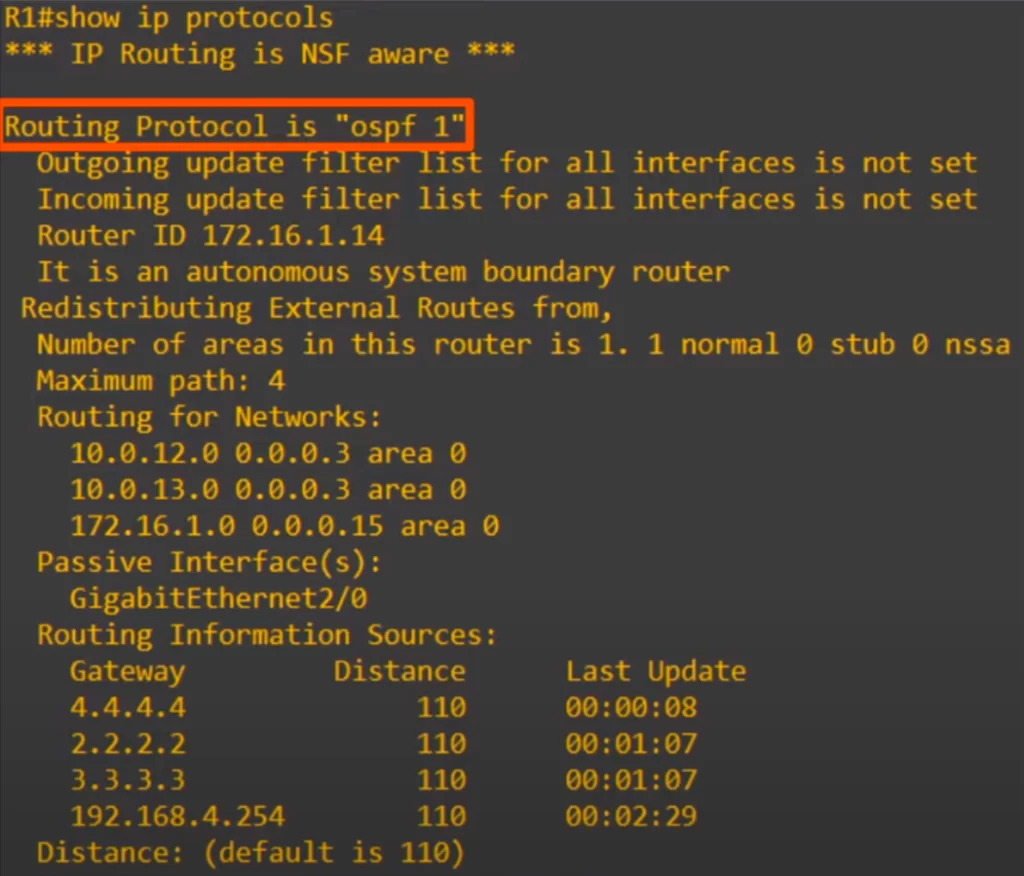
Up top it says Routing Protocol is ospf 1. “1” is the process ID we configured earlier. 

OSPF also uses a router ID. The router ID is determined in exactly the same way as in EIGRP. Let’s review it. 

Here is the order of priority when determining the OSPF router ID.

1) Manual configuration. If you manually configure the router ID, that will become the router ID.

2) Highest IP address on a loopback interface. If you do not manually configure the router ID, the highest IP address on a loopback interface will become the router ID. 

3) Highest IP address on a physical interface. If the router has no loopback interfaces with an IP address, the highest IP address on a physical interface will become the router ID. 

Currently R1’s router ID is 172.16.1.14, because we have not manually configured the router ID, and also we have not configured a loopback interface on R1.

Let’s see how to manually configure the router ID.

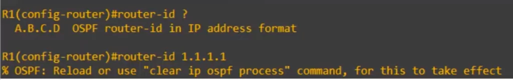
From OSPF configuration mode, use the router-id command. This is a little different from EIGRP. In EIGRP the command is eigrp router-id.

We entered a router ID of 1.1.1.1, but then the router displayed this message: “Reload or use ‘clear ip ospf process’ command, for this to take effect”.

Currently, the router ID is still 172.16.1.14. To make 1.1.1.1 take effect we have to either reload the router or use the clear ip ospf process command to clear the OSPF process and reset it. 

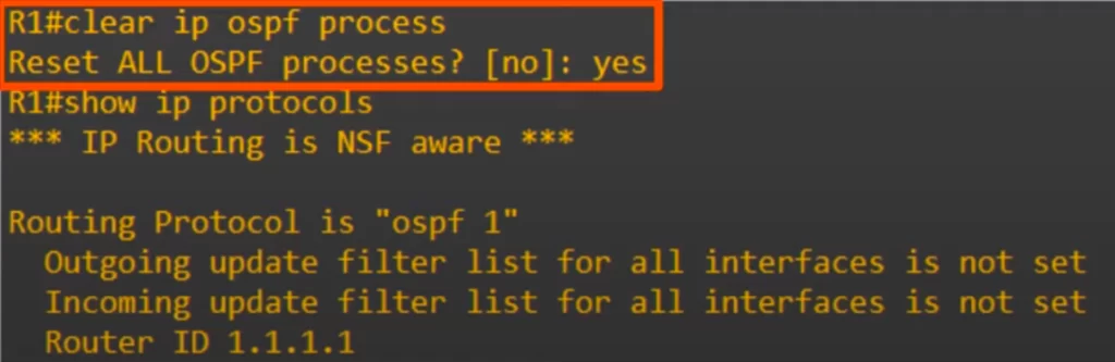
Let’s use the command clear ip ospf process from privileged EXEC mode which basically resets OSPF on the router. 

But this is a bad idea in a real network, and the router will lose all of its OSPF routes for a short time and will not be able to forward traffic to those destinations. 

Using show ip protocols again shows that the router ID is now 1.1.1.1.

Let’s continue exploring the rest of the CLI output for the command show ip protocols.

*Notice the entry, “It is an autonomous system boundary router”.

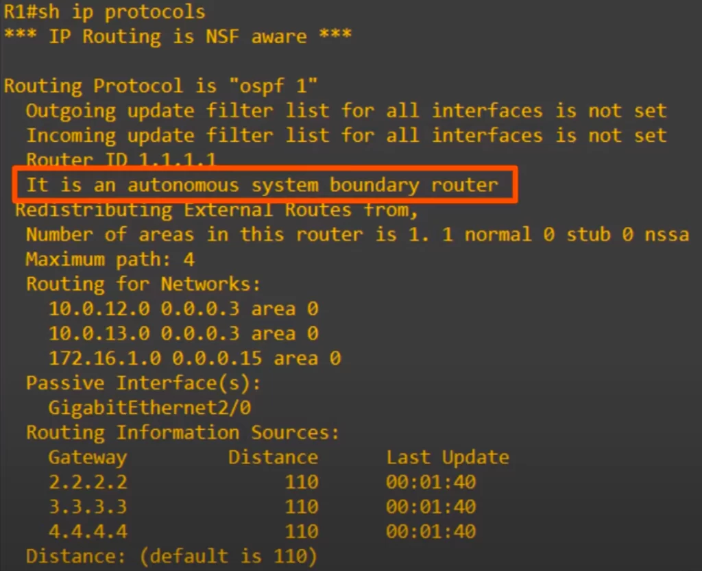
An autonomous system boundary router (ASBR) is an OSPF router that connects the OSPF network to an external network. By using the default-information originate command, R1 becomes an ASBR, connecting the OSPF network to the Internet. That’s why we see the output “It is an autonomous system boundary router” on R1.

*Next up, “Number of areas in this router is 1. 1 normal 0 stub 0 nssa”. These are three different types of OSPF areas. For the CCNA, we are just interested in knowing the number of areas this router is in, i.e., 1, because this is single-area OSPF. 

*Next, maximum paths is 4. Unlike EIGRP, OSPF does not support unequal-cost load-balancing, but it does support ECMP (Equal-Cost Multi-Path) load-balancing over a maximum of 4 paths by default. To change the maximum number of paths, use the command maximum-paths, just like in RIP and EIGRP. Here we changed the number to 8. 

R1(config-router)#maximum-paths ?

<1-32> Number of paths

R1(config-router)#maximum-paths 8

*Next up, the Routing for Networks section shows the network commands we used. This only determines which interfaces OSPF will be activated on.

*Next, notice the passive interface configured, GigabitEthernet2/0.

*Next, are R1’s neighbors under Routing Information Sources. Notice the router IDs – these loopback interfaces were configured on R2, R3, and R4 and their IP addresses became the router IDs. 

*Finally, OSPF’s AD is displayed (Distance). The default is 110. If you want to change it, the command is the same as for RIP and EIGRP. From OSPF configuration mode, use the command distance. For example, it was changed to 85, so OSPF routes are preferred over EIGRP routes on this router.

R1(config-router)#distance ?

<1-255> Administrative distance

R1(config-router)#distance 85

Command review

>Configure ospf on a router:

R(config)#router ospf process-id
→to enter OSPF configuration mode

R(config-router)#network network-address wildcard-mask area area-number

>Configure a passive interface:

R(config-router)#passive-interface interface

R#show ip protocols
→to check if ospf is running, router ID, load balancing paths, advertised ospf networks, and passive interfaces

>Advertise a default route into ospf:

Step 1. R(config)#ip route 0.0.0.0 0.0.0.0 next-hop
→configure a default route

Step 2. R(config-router)#default-information originate 
→to advertise the default route into OSPF 

Step 3. R#show ip route
→to verify the configs

>Manually configure router ID:

R(config-router)#router-id router-id

>To reset ospf process (to change router ID):

R#clear ip ospf process

>Change ECMP load balancing (default is 4 paths maximum):

R(config-router)#maximum-paths number-of-paths

>Change AD (default is 110):

R(config-router)#distance AD

Free CCNA | Configuring OSPF (1) | Day 26 Lab – Notes

Key learnings

*An overview of OSPF operations, including LSA flooding and neighbor discovery using hello messages. OSPF operations refer to tasks that are performed by OSPF routers in order to maintain a routing table and route traffic between networks.

*Basic OSPF rules and concepts related to OSPF areas, including ABR and ASBR. 

*Basic OSPF configurations for R1, including:

• How to configure OSPF on R1 using the network command from ospf configuration mode.
• How to configure G2/0 as a passive interface using the passive-interface command and then verify the configuration with the show ip protocols command.
• How to configure a default route 0.0.0.0/0 via gateway 203.0.113.2 using the ip route command and confirm the configuration in the routing table with the show ip route command.
• How to advertise a default route into OSPF using the command default-information originate and confirm the configuration with show ip route on R2 (an R1 OSPF neighbor).
• How to manually configure a router ID on R1 using the router-id command and verify the configuration using the show ip protocols command.

Most of these were the same as in RIP and EIGRP, with a few minor differences.

Practice quiz questions

Quiz question 1

Which of the following statements about OSPF are not true? Select two. 

A. In multi-area OSPF networks, all non-backbone areas must have an ABR connected to area 0.

B. Single-area OSPF must use area 0. 

C. Two OSPF routers with different process IDs can become OSPF neighbors.

D. The OSPF area must be specified in the network command.

E. An ASBR connects the internal OSPF network to networks outside of the OSPF domain.

F. The OSPF process ID must match the area number.

The answers are B and F. The other statements are all true.

Quiz question 2

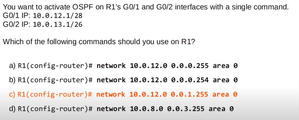
The answer is C. This is the only option that contains both IP addresses in its range, so it is the only one that activates OSPF on both interfaces.

G0/1 IP	10	0	00001100	1
G0/2 IP	10	0	00001101	1
Network command (C)	10	0	00001100	0
Wildcard mask	0	0	00000001	255

You can find three more practice quiz questions (plus a bonus one) for this lesson in Jeremy’s OSPF Part 1 video, cited below.

Key references

Note: The resources cited below (in the “Key references” section of this document) are the main source of knowledge for these study notes/this lesson, unless stated otherwise.

Free CCNA | OSPF Part 1 | Day 26 | CCNA 200-301 Complete Course

Free CCNA | Configuring OSPF (1) | Day 26 Lab | CCNA 200-301 Complete Course

Related content

CCNA 200-301 study notes

Compliance frameworks and industry standards

How data flow through the Internet

How routers become OSPF neighbors

How to break into information security

How to get CCNA certification

IT career paths – everything you need to know

Job roles in IT and cybersecurity

Key CCNA terms and concepts

Network security risk mitigation best practices

OSPF network types

The GRC approach to managing cybersecurity

The penetration testing process

The Security Operations Center (SOC) career path

What do ethical hackers do?

Back to DTI Courses