This lesson kicks off a series of lessons on dynamic routing. This lesson introduces dynamic routing protocols types, algorithms, and metrics. The lesson on routing fundamentals covered connected and local routes – these are automatically added in the routing table when you configure IP addresses on router interfaces. The lesson on static routing introduced static routes and looked at how to configure static routes in the CLI of Cisco routers. Unlike Connected and Local routes, static routes must be manually configured on the router.
This lesson first gives a general overview of dynamic routing protocols to demonstrate how they function and why they are usually preferred over static routes. Then the types of dynamic routing protocols are discussed. Then we go over dynamic routing protocol metrics. Finally, we talk about administrative distance (AD). Beside metric, AD is part of the mechanism of determining the best route to a destination.
This and the next few lessons cover a large portion of the CCNA exam topics list. Section 3.0, IP Connectivity, accounts for 25% of the CCNA exam, and we’re going to cover almost all of it over this and the next few lessons. The next lesson covers RIP (Routing Information Protocol) & EIGRP (Enhanced Interior Gateway Routing Protocol) and it is followed by three lessons on OSPF (Open Shortest Path First). OSPF is actually the only dynamic routing protocol explicitly named in the CCNA exam topics list, in subsection 3.4. This post constitutes Issue 19 of my CCNA 200-301 study notes.
- Network topology
- Network route/host route
- Dynamic routing
- Dynamic vs static routing
- Dynamic routing summary
- Dynamic routing protocol types
- IGP/EGP algorithm types
- Distance vector routing protocols characteristics
- Link state routing protocols characteristics
- Dynamic routing protocols metrics
- ECMP with static routes
- IGP metric chart
- Administrative distance (AD)
- Configure AD of a static route
- Floating static routes
- Command review
- Key learnings
- Key references
You may also be interested in CCNA 200-301 study notes.
Network topology
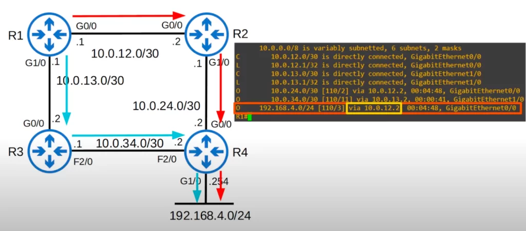
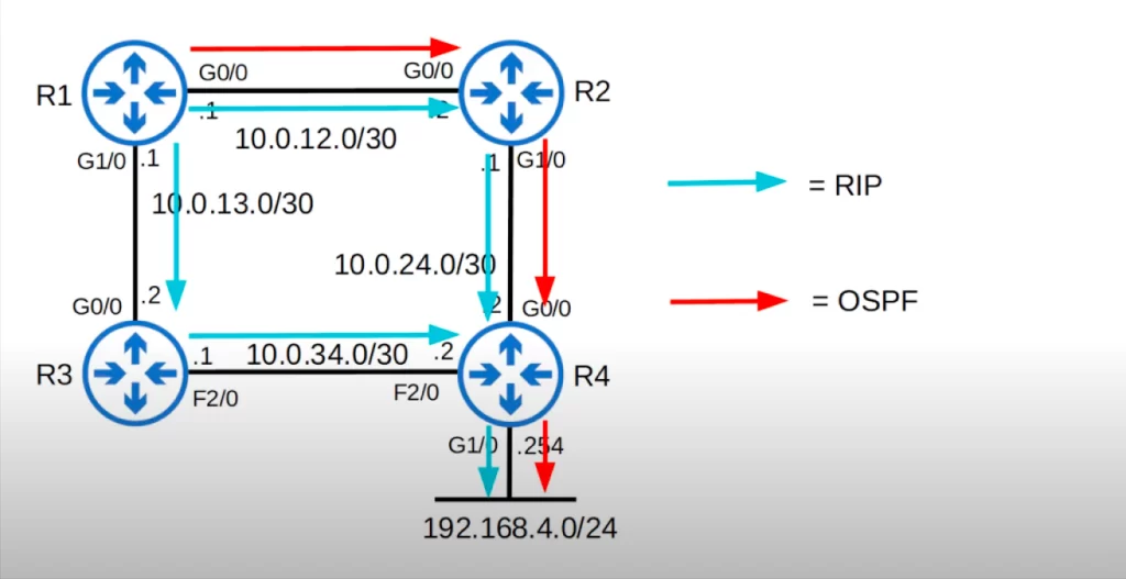
We will use the following network topology for this lesson. There are four routers, R1, R2, R3, and R4, and there is a LAN connected to R4, 192.168.4.0/24. We will be focusing mostly on R1’s perspective for now.
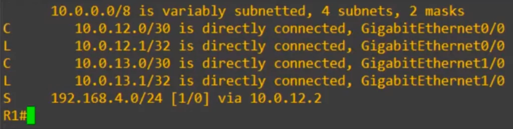
Without configuring any static routes or dynamic routing protocols, R1’s routing table looks like this (use the command show ip route to view the routing table). Connected and local routes were automatically added to the routing table when IP addresses were configured on R1’s interfaces.
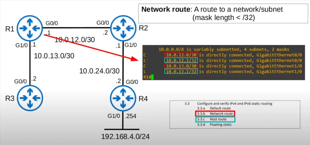
Connected routes provide a route to a network the router’s interface is directly connected to, and Local routes provide a route to the router’s own IP address.
Network route/host route
The two routes, 10.0.12.0/30 and 10.0.13.0/30, are examples of network routes. A network route is a route to a network or subnet. In other words, a route with a mask length less than /32. For example, if we configure a static route to 192.168.4.0/24, that’s a network route also. It’s not a route to a single host, but a route to a whole subnet, meaning a route that matches all of the IP addresses in a subnet.
A host route has a prefix length of /32, which means that it only matches a single IP address.
Another example, a network route to the subnet 192.168.1.0/24 would match all of the IP addresses in that subnet, such as 192.168.1.1, 192.168.1.2, and so on (in a /24 network the first three octets in the IP address are fixed). A host route to the IP address 192.168.1.1 would only match that single IP address.
The two routes, 10.0.12.1/32 and 10.0.13.1/32, are examples of host routes. A host route is a route to a specific host, a single address, specified with a /32 mask. These two routes were automatically added, and are host routes to the specific addresses configured on R1’s G0/0 and G1/0 interfaces.
To configure a static route to a host, use IP ROUTE, followed by the host’s address, then 255.255.255.255, which is a /32 mask, then the next-hop IP address.
Dynamic routing
While static routing involves manually configuring routes to each destination, dynamic routing involves configuring a dynamic routing protocol on a router and then letting the router take care of finding the best routes to destination networks. Dynamic routing is so called because it is not fixed. If you add a new LAN, routers will automatically inform each other about how to get to that new destination network. If one path to a destination becomes unavailable, the routers will automatically start using the next best path.
Instead of configuring static routes on each of the routers in the following diagram, we can enable a dynamic routing protocol on them. Then, R4 will advertise the 192.168.4.0/24 network to its neighbor R2, telling R2 “you can reach 192.168.4.0/24 via me”.
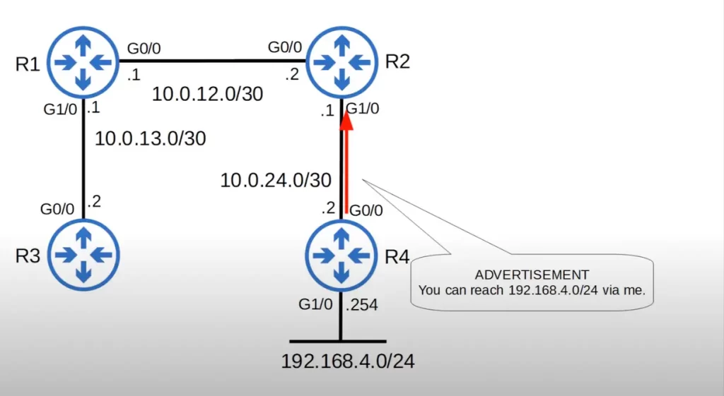
R2 will add that route to its route table. R2 will then advertise the same route to R1, telling R1 that it (R1) can reach 192.168.4.0/24 via R2. R1 will add this route to its route table.
You can see in the following CLI output of R1’s routing table that R2 also advertised the 10.0.24.0/30 network between R2 and R4 to R1, and R1 added it to its route table. Note, “O” stands for OSPF. OSPF is a routing protocol that is used to dynamically distribute routing information between routers.
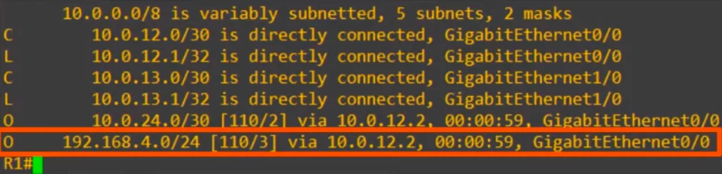
R1 will then in turn advertise to R3, telling R3 that it can reach 192.168.4.0/24 via R1. R1 will also advertise the 10.0.24.0/30 network that it learned from R2, as well as the 10.0.12.0/30 network between R1 and R2.
If R4’s G0/0 interface went down due to some malfunction, the other routers will automatically adapt and remove the route from their route tables. This prevents R1 from continuously sending traffic to a dead-end.
Dynamic vs static routing
We configured a static route on R1 (note the letter “S” for static in the following CLI output). R1 can send traffic to R4’s network with no problems.
Because there is no dynamic routing protocol in use, if R4’s G0/0 interface goes down, R1 will remain unaware that it can no longer reach the 192.168.4.0/24 network. If R1 receives packets destined for that network, it will continue forwarding them to R2, unaware that R2 can no longer reach the network.
Dynamic routing (cont.)
To achieve redundancy in the network, ideally we want to have more than one route for R1 to reach R4, a backup route for the preferred route.
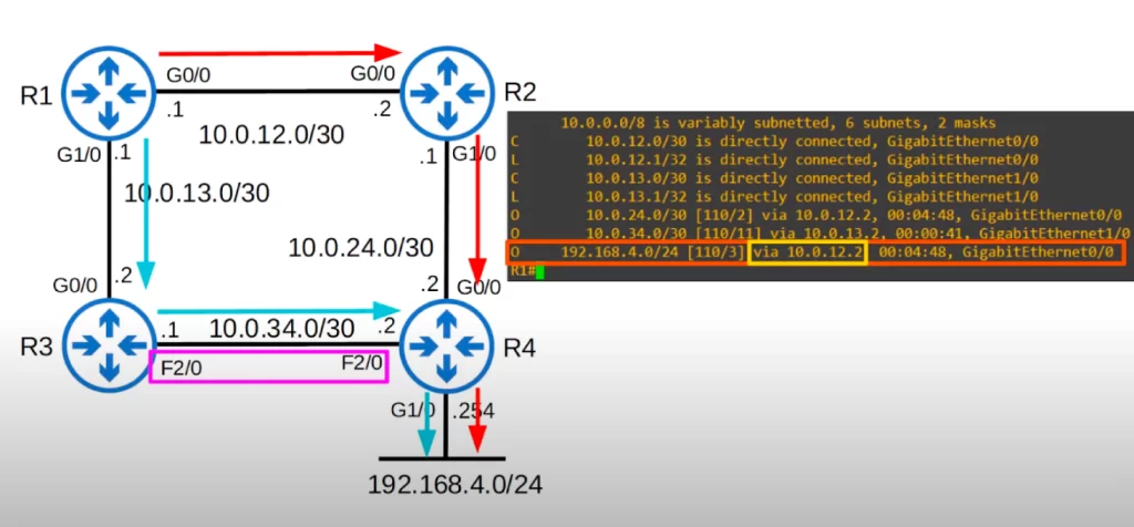
A connection between R3 and R4 has been added. Now R1 has two valid paths to R4’s internal network, via R2 and via R3. OSPF is enabled on the routers. Let’s check R1’s route table. You can see, R1 has the route via R2 in its route table, via 10.0.12.2.
What will happen if we disable R4’s G0/0 interface to simulate a failure?
We did that, and now let’s check R1’s route table.
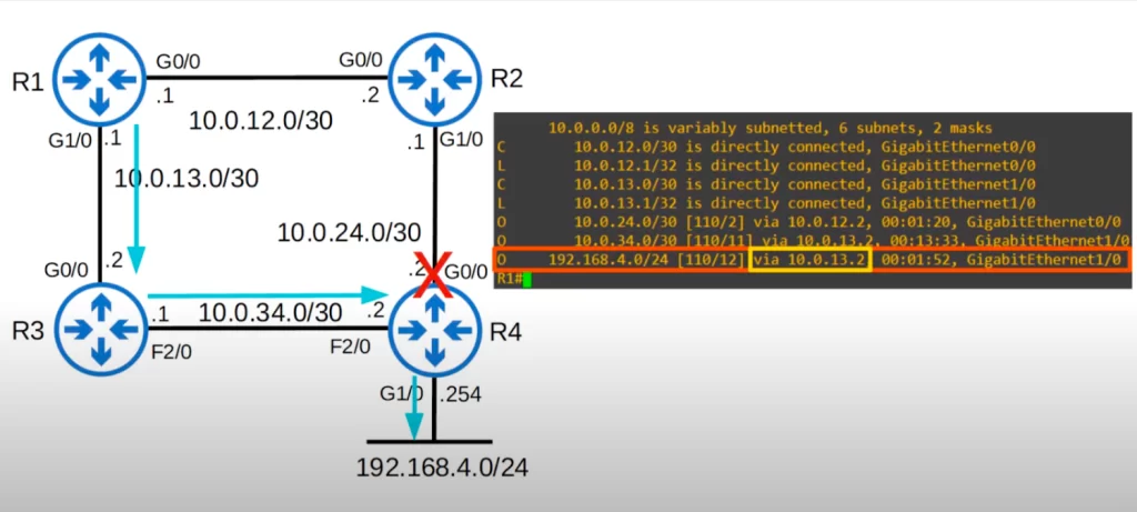
As you can see, the route via R2 was now automatically replaced with the route via R3, 10.0.13.2. So we lost the preferred route to 192.168.4.0, but traffic can still follow this other path.
The route via R2 was preferred over the route via R3 because the connection between R3 and R4 is a FastEthernet connection, while the connection between R2 and R4 is Gigabit Ethernet. In Spanning Tree Protocol (STP), root cost is used to determine the best path to the root bridge. Dynamic routing protocols use a similar concept to determine the best path to a destination. R1 learned about the 192.168.4.0/24 network from both R2 and R3, however it determined that the path via R2 is superior because it costs less.
Dynamic routing summary
*Routers use dynamic routing protocols to advertise information about their connected routes and about routes they learned from other devices.
*Routers form adjacencies also known as neighbor relationships or neighborships with adjacent routers to exchange this information. For example, in our demo network topology R1 will form adjacencies with R2 and R3, its directly connected neighbors.
*If multiple routes to a destination are learned, the router determines which route is superior and adds it to the routing table. Routers use the metric of the route to decide which route is superior, and the lower metric is superior. Just like in Spanning Tree, the lower root cost is superior when determining the root port on a switch.
Dynamic routing protocol types
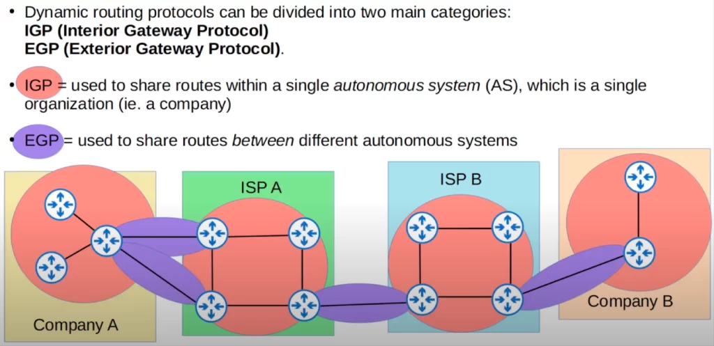
Dynamic routing protocols can be divided into two main categories:
1) IGPs or Interior Gateway Protocols, used to share routes within a single autonomous system (AS), which is a single organization (e.g., a company).
2) EGPs or Exterior Gateway Protocols, used to share routes between different autonomous systems, for example, over the Internet.
Here is a diagram to help clarify the concepts. Company A (ISP A) and Company B (ISP B) are each their own autonomous system. Within each organization, an IGP is used to exchange routing information. However, to exchange routing information between autonomous systems, an EGP is used.
The basic purpose of IGPs and EGPs is the same, to share information about routes to destinations. However they function differently.
This discussion focuses on OSPF because it is the only dynamic routing protocol explicitly named in the CCNA exam topics list.
IGP/EGP algorithm types
Let’s break down these two categories of dynamic routing protocols, IGP and EGP, further by algorithm type. Algorithms refer to the processes each protocol uses to share route information and determine the best route to each destination.
Here is a chart of the different kinds of routing protocols.
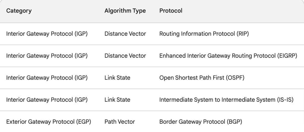
All routing protocols have the same goal, to share route information and select the best route to each destination. However, the algorithm used to do so is different for each routing protocol.
There are two kinds of IGP algorithms:
- distance vector, used by RIP (Routing Information Protocol) and EIGRP (Enhanced Interior Gateway Routing Protocol), and
- link state, used by OSPF (Open Shortest Path First) and IS-IS (Intermediate System to Intermediate System).
There is one type of EGP algorithm, path vector, used by BGP (Border Gateway Protocol).
Remember the names of each of these routing protocols. And remember which protocols use which kind of algorithm.
Here’s a mnemonic for IGP algorithms: DR DE, LO LI.
D stands for Distance vector, and L stands for Link state.
DR can be unpacked as “distance vector RIP”. DE can be unpacked as “distance vector EIGRP”. LO refers to “link state OSPF”. And LI refers to “link state IS-IS”.
Distance vector routing protocols characteristics
*Distance vector protocols were invented in the early 1980s, before link state protocols.
*Early examples of distance vector protocols are RIPv1 and Cisco’s proprietary protocol IGRP, which was later updated to become EIGRP.
*Distance vector protocols operate by sending the following information to their directly connected neighbors: their known destination networks, and their metric to reach their known destination networks. Each router shares information about the routes they know and their metric cost to reach each destination.
*This method of sharing route information is often called routing by rumor because the router does not know about the network beyond its neighbors. The router only knows the information that its neighbors tell it.
*Distance vectors are so-called because the routers only learn the distance, which is the metric, and the vector, which is the direction to send the traffic, the next-hop router, of each route.
The example we saw earlier of R4 advertising its 192.168.4.0/24 network is an example of distance vector logic.
Note that OSPF is considered primarily a link state routing protocol. However, when OSPF spans multiple areas, it uses a distance vector approach between these areas. This is done to prevent routing loops and maintain scalability. But within each OSPF area, OSPF remains a link state protocol.
R4 tells its directly connected neighbor R2, “you can reach 192.168.4.0/24 via me. My metric to reach it is 1.” Each routing protocol uses a different type of metric.
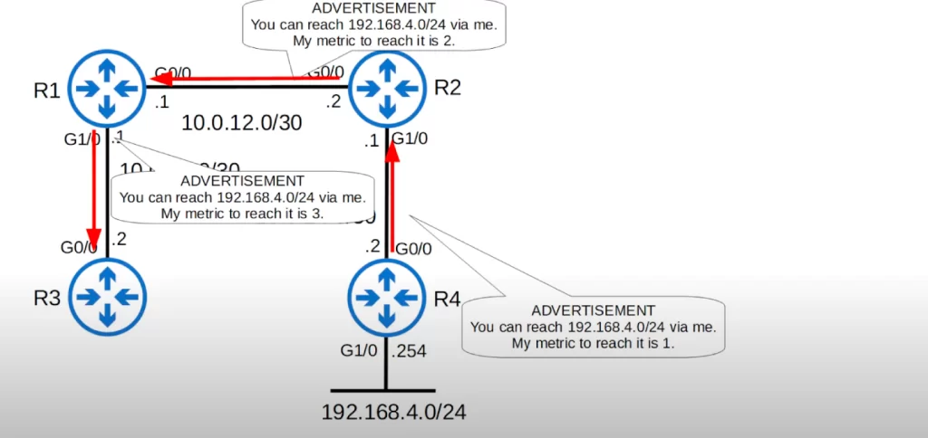
R2 does not know anything except that it can reach 192.168.4.0/24 via R4, and that R4’s metric is 1. Similarly, R2 then tells R1 that R1 can reach 192.168.4.0/24 via R2 and that R2’s metric for this route is 2. Again, R1 does not have a detailed picture of the network, all R1 knows is that it can reach 192.168.4.0/24 via R2, and that R2’s metric to reach it is 2. R1 advertises the network to R3, with its own metric to reach the destination network.
Link state routing protocols characteristics
*When using a link state routing protocol, every router creates a connectivity map of the network. This map will be the same on each router.
*To allow this, each router advertises information about its interfaces (connected networks) to its neighbors. These advertisements are passed along to other routers, until all routers in the network develop the same map of the network.
*Then each router independently uses this map to calculate the best routes to each destination. In link state protocols, each router gets a whole picture of the network so that it can calculate the best routes.
*Link state protocols use more resources on the router (more CPU power and memory) than distance vector protocols because more information is shared.
*However, link state protocols tend to be faster in reacting to changes in the network than distance vector protocols.
Dynamic routing protocols metrics
*A protocol’s metric is how it measures how far is the destination, and it’s used to determine the best route to a destination.
The purpose of all routing protocol metrics is the same, to let the router select the best route to the destination, but some routing protocols might make better decisions than others.
*A router’s route table contains the best route to each destination network it knows about.
*If a router using a dynamic routing protocol learns two different routes to the same destination it will use the metric value of the routes to determine which route is the best.
A lower metric is considered better. It is like the root cost in Spanning Tree. A lower root cost is considered superior, so the interface with the lowest root cost will become the root port. For dynamic routing protocols, the route with the lowest metric is considered best and will be entered into the routing table.
*Each routing protocol uses a different metric to determine the best route to a destination.
Although R1 learns two paths to 192.168.4.0/24, one via R2 and one via R3, only the route via R2 is added to the routing table.
The FastEthernet connection between R3 and R4 has a higher metric cost than the Gigabit Ethernet connection between R2 and R4, so the route via the FastEthernet connection is less favorable.
What if the connection between R3 and R4 was also a Gigabit Ethernet connection? Both routes would have the same cost, so which route would be added to the route table?
Let’s see what happens.
The connection between R3 and R4 was changed to be a Gigabit Ethernet connection. Let’s check out R1’s route table.
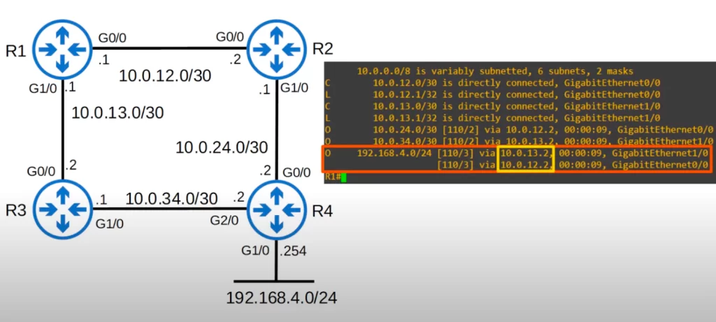
Both routes have been added to the table: via 10.0.13.2, which is R3, and via 10.0.12.2, which is R2.
If a router learns two (or more) routes via the same routing protocol to the same destination (same network address, same subnet mask), with the same metric, both routes will be added to the routing table. Traffic will be load-balanced over both routes. Note that they must be exactly the same destination, the same network address, and same prefix length.
Here’s a larger view of R1’s routing table. Both routes were learned by the dynamic routing protocol OSPF, as indicated by the code O next to the routes. They are both to the exact same destination, 192.168.4.0/24, and they both have the same metric.
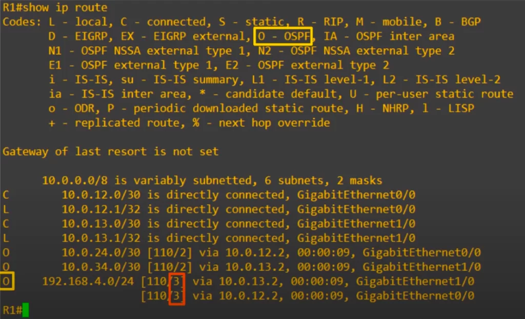
The metric value is displayed in the output. The second value in the square brackets (in the red square) is the metric value of the route. Both routes have a metric of 3, so both routes were added, and traffic will be load-balanced over both routes. This type of load-balancing is called Equal Cost MultiPath load-balancing or ECMP load-balancing.
The values on the left side of the square brackets (110), are administrative distance (AD) values. The OSPF protocol has an AD of 110.
ECMP with static routes
We just saw ECMP with a dynamic routing protocol. Let’s see ECMP done with static routes.
OSPF was disabled on R1 and two static routes to 192.168.4.0 were configured, one via R2 and one via R3. Traffic will be load-balanced over both routes.
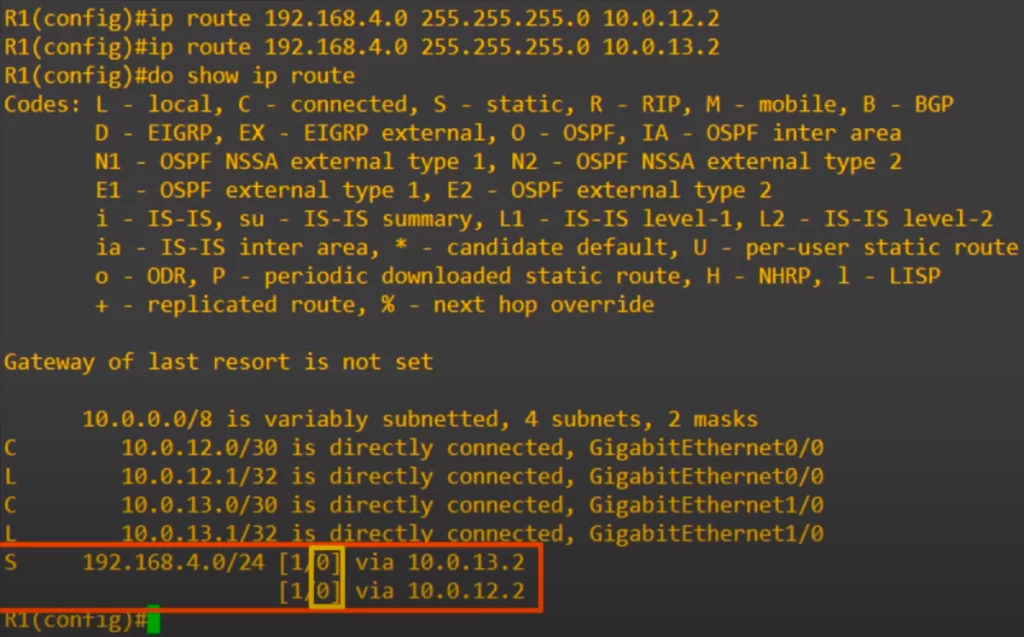
Notice, both routes have a metric of 0. Static routes do not use the concept of metric so you will always see 0 for them. Notice also that the AD value of static routes is 1. The connected and local routes above them have an AD of 0, but it is not displayed in the route table.
IGP metric chart
Each routing protocol uses a different metric, which is a value used to determine the best route to a destination. Here is a summary introducing each metric.
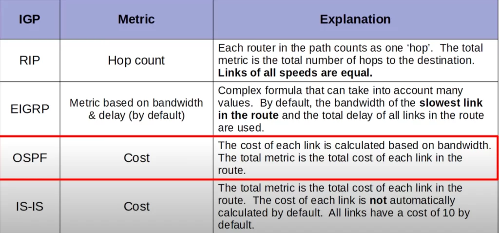
RIP uses the simplest metric, hop count. Each router in the path to the destination counts as one hop, and the total metric is the total number of hops to reach the destination. One big downside is that links of all speeds are equal, they all count as one hop. A 10 Mbps Ethernet link is one hop, and a 10 Gigabit per second link is one hop.
EIGRP uses the most complicated metric of the IGPs, which is a calculation based on bandwidth and delay by default, however with configuration other factors can be calculated as well. By default, only the bandwidth of the slowest link in the route is used to calculate the metric, beside the total delay values of all links in the path. This delay value is a little misleading, since by default it’s a value assigned to the interface based on its bandwidth.
OSPF’s metric is called cost. The cost of each link is calculated based on the bandwidth, and the total bandwidth of the links in the route make up the metric of the route. This is a very simple way of calculating metric, but also clearly better than RIP’s which does not take into account link speed.
IS-IS also uses a metric called cost. However, the cost of each link is not automatically calculated based on bandwidth. All links have a cost of 10 by default. So, without any configuration, it functions the same as RIP, being a simple hop count metric.
Remember RIP uses hop count, EIGRP uses a calculation based on bandwidth and delay, and OSPF uses a cost based on bandwidth.
To demonstrate how the difference in metrics can affect which routes the router selects, let’s return to our network topology. R1 has to decide which route to 192.168.4.0/24 to select for its route table. If R1 uses RIP, the metric is hop count. Via R2, the hop count is 2. One hop to R2, one hop to R4. Via R3, the hop count is also 2. One hop to R3, one hop to R4, even though the connection from R3 to R4 is a slower Fastethernet connection. So, both routes will be added to R1’s route table, and R1 will load balance traffic using both routes, even though one route is slower.
However, if OSPF is used instead of RIP, which path will be used? Unlike RIP, OSPF’s metric cost takes into account bandwidth. The slower connection between R3 and R4 will result in a higher metric value, making it less favorable. So only the route via R2 will be entered into the route table, and R1 will send all traffic destined to the 192.168.4.0/24 network via R2.
Administrative distance (AD)
*Metric is used to compare routes learned via the same routing protocol. If a router learns two routes to the same destination via OSPF, it uses a metric to choose which route is better.
*However, different routing protocols use totally different metrics, so they cannot be compared.
For example, an OSPF route to a network, say, 192.168.4.0/24, might have a metric of 30, while an EIGRP route to the same network might have a metric of 33280. Which route is better? Which route should the router put in the route table? We cannot really answer those questions by looking at the metrics, because OSPF and EIGRP use totally different metrics.
*If a router receives routes to the same destination from different routing protocols, administrative distance (AD) is used first to select the best route.
When a router receives multiple routes to the same destination from different routing protocols, the router first compares the ADs of the routes. The route with the lowest AD is considered to be the best route. If two routes have the same AD, the router then compares the metrics of the routes. The route with the lowest metric is considered to be the best route.
*The AD is used to determine which routing protocol is preferred. A lower AD is preferred, and indicates that the routing protocol is considered more trustworthy, meaning more likely to select good routes. As we saw, RIP’s hop count-based metric system is not very good, so RIP has a high AD, because RIP is not very trustworthy. RIP might say two routes are equal because they have the same hop count, although really one route is much worse because of lower bandwidth.
*In most cases a company will only use a single IGP for its network – usually OSPF, but sometimes EIGRP if the company only uses Cisco equipment.
*Less often a company might use two dynamic routing protocols. For example, if two companies connect their networks to share information, two different routing protocols might be used. You might connect a network running OSPF to a network running EIGRP.
AD is a measure of the trustworthiness of the source of the routing information. For example, OSPF is a more reliable protocol than RIP, so OSPF routes are assigned a lower AD value than RIP routes. This means that OSPF routes will be preferred over RIP routes when there are multiple routes to the same destination. Routes with lower AD values are preferred over routes with higher AD values.
Ready for some memorization? The default AD values for some common routing protocols are as follows:
| Route protocol/type | AD |
| Directly connected | 0 |
| Static | 1 |
| External BGP (eBGP) | 20 |
| EIGRP | 90 |
| IGRP | 100 |
| OSPF | 110 |
| IS-IS | 115 |
| RIP | 120 |
| EIGRP (external) | 170 |
| Internal BGP (iBGP) | 200 |
| Unusable route | 255 |
You are likely to get a question on the CCNA exam along these lines: two routes to the 10.0.0.0/24 network are learned, one from OSPF and one from EIGRP. Which route will be entered in the route table? To answer this question, you would need to know that EIGRP has a lower AD, so the EIGRP route is preferred and will be entered in the route table.
Keep in mind that these are the values used on Cisco devices, other vendors might rank these protocols for ADs differently.
So the most preferred routes are those to directly connected networks, they have an AD of 0. Static routes are the next best, they have an AD of 1.
Of the IGPs we saw, which are RIP, EIGRP, OSPF, and IS-IS, EIGRP is the most preferred since it has the lowest AD. However, EIGRP external routes have a higher AD, 170. These are beyond the scope of the CCNA, but basically they are routes from outside of the EIGRP network that are then advertised into EIGRP.
Routes with an AD of 255 are unusable. Here’s a quote from Cisco: “If the administrative distance is 255, the router does not believe the source of that route and does not install the route in the routing table.”
Configure AD of a static route
*You can change the AD of a routing protocol. If you want OSPF routes to be preferred over EIGRP routes, you can configure the router to do that.
*You can also change the AD of a static route. Here is how.
Use the standard command to configure a static route: IP ROUTE, followed by the destination, the subnet mask, and then the next hop address. And then the AD value we want to configure.
In our example below, we first used the question mark to check for further options.
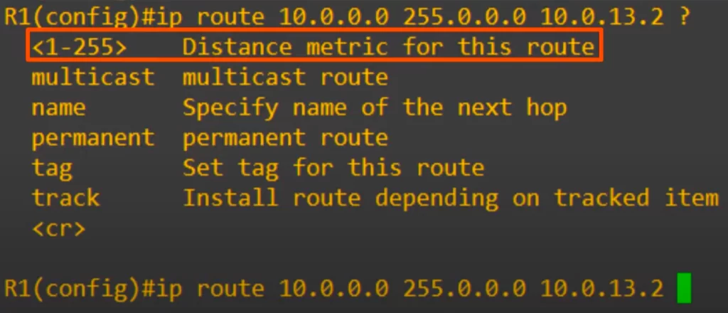
Note, the “Distance metric for this route” option refers to administrative distance.
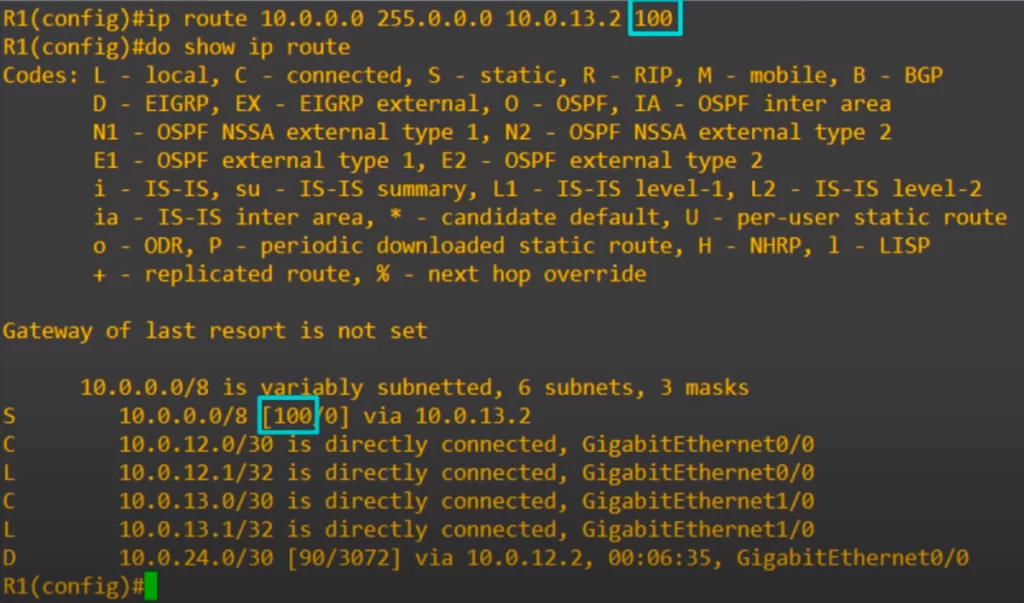
We configured the route with an AD of 100.
In the output of show ip route, you can see that the AD is now 100, instead of the default 1 for a normal static route. We thus made this static route less preferred.
Floating static routes
*By changing the AD of a static route, you can make it less preferred than routes learned by a dynamic routing protocol to the same destination.
*This kind of static route is called a floating static route. Floating static routes are part of the CCNA exam topics list:
3.0 IP Connectivity
3.3 Configure and verify IPv4 and IPv6 static routing
3.3.a Default route
3.3.b Network route
3.3.c Host route
3.3.d Floating static
*The route will be inactive, meaning it will not be in the routing table, unless the route learned by the dynamic routing protocol is removed (maybe the router stops advertising the dynamic route for some reason, or an interface failure causes an adjacency with a neighbor to be lost).
Command review
>To configure a static route to a host:
R(config)#ip route dst-host-ip-address 255.255.255.255 next-hop-ip-address
>To configure static route to a network:
R(config)#ip route dst-network-ip-address subnet-mask next-hop-ip-address [AD]
By changing the AD of a static route, you can make it less preferred than routes learned by a dynamic routing protocol to the same destination. This kind of static route is called a floating static route.
Free CCNA | Floating Static Routes | Day 24 Lab – Notes
Key learnings
*What are dynamic routing protocols.
*Types of dynamic routing protocols, broken down by algorithm type.
*Dynamic routing protocols metrics, focusing on RIP, EIGRP, OSPF, and IS-IS.
*Administrative distance of each kind of route and routing protocol.
Key references
Note: The resources cited below (in the “Key references” section of this document) are the main source of knowledge for these study notes/this lesson, unless stated otherwise.
Free CCNA | Dynamic Routing | Day 24 | CCNA 200-301 Complete Course
Free CCNA | Floating Static Routes | Day 24 Lab | CCNA 200-301 Complete Course
Related content
Compliance frameworks and industry standards
How data flow through the Internet
How to break into information security
IT career paths – everything you need to know
Job roles in IT and cybersecurity
Network security risk mitigation best practices
The GRC approach to managing cybersecurity
The penetration testing process
The Security Operations Center (SOC) career path
Back to DTI Courses