This is Part 2 of 3 of OSPF study notes for the CCNA exam. OSPF Part 1, Basic OSPF operations, introduces the basic functions of OSPF and covers the basics of configuring single area OSPFv2. More specifically, OSPF Part 1 covers how to configure OSPF on a router, how to configure a passive interface on a router, how to advertise a default route into OSPF, and how to manually configure a router ID on a router.
OSPF Part 3, OSPF network types, covers the role and election of designated and backup designated routers in a subnet, how to configure the OSPF interface priority on a router in an OSPF broadcast network, how to configure the clock rate on the DCE side of a serial connection, how to configure PPP encapsulation on a point-to-point router, how to manually configure the OSPF network type of an interface on a router, OSPF neighbor/adjacency requirements (troubleshooting adjacency problems), and the role of Type 1, Type 2 and Type 3 LSAs in IP connectivity within OSPF areas.
This lesson, OSPF Part 2 , focuses on the calculation and configuration of OSPF’s metric (cost) and on the process of how routers become OSPF neighbors. More specifically, this lesson covers the seven OSPF neighbor states, three methods to change the OSPF cost, how to configure OSPF directly on a router interface, and how to configure passive OSPF interfaces. This post constitutes Issue 22 of my CCNA 200-301 study notes.
- OSPF’s metric (cost)
- Changing the reference bandwidth
- OSPF cost summary
- OSPF neighbors
- OSPF neighbor states (7 states)
- How routers become OSPF neighbors (summary)
- OSPF message types chart
- OSPF show commands
- OSPF configurations cont.
- Command review
- Key learnings
- Practice quiz questions
- Key references
You may also be interested in CCNA 200-301 study notes.
OSPF’s metric (cost)
*OSPF’s metric is called cost. OSPF’s cost is automatically calculated based on the bandwidth (speed) of the interface. You can also manually configure the cost of each interface.
*The interface’s cost is calculated by dividing a value called the reference bandwidth by the interface’s bandwidth. The default OSPF reference bandwidth is 100 megabits per second (mbps).
Example 1: a regular Ethernet interface with a speed of 10 mbps has an OSPF cost of 10, because 100 divided by 10 equals 10. Reference / Interface = 100 mbps / 10 mbps = cost of 10.
Example 2: a FastEthernet interface with a speed of 100 mbps has an OSPF cost of 1, because 100 divided by 100 is 1. Reference / Interface = 100 mbps / 100 mbps = cost of 1.
A Gigabit Ethernet interface with a speed of 1000 mbps has a cost of 1, even though 100 divided by 1000 equals 0.1.
A 10 Gig Ethernet interface with a speed of 10000 mbps also has a cost of 1, even though 100 divided by 10000 equals 0.01.
How come?
*In OSPF, all cost values less than 1 will be converted to 1. Therefore FastEthernet, Gigabit Ethernet, 10 Gig Ethernet, etc. are all equal and all have a cost of 1 by default.
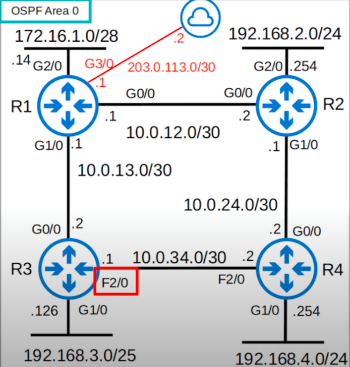
Let’s look at the CLI. Here is the same network topology as before (from OSPF Part 1). Let’s check the cost of R3’s F2/0 interface using the command show ip ospf interface. The cost is 1. The cost is displayed in two places.
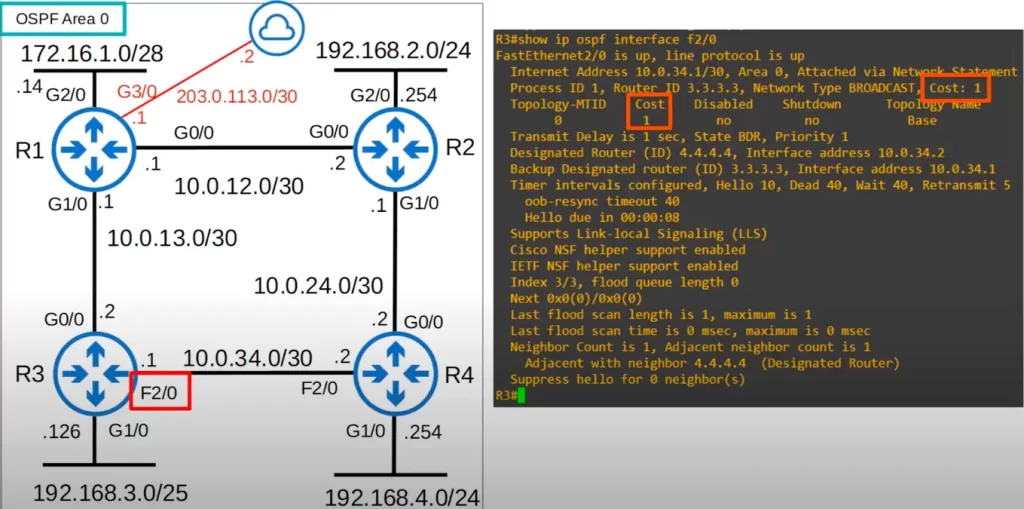
The default cost of a FastEthernet interface is 1, because FastEthernet operates at a speed of 100 mbps and the reference bandwidth is 100 mbps by default.
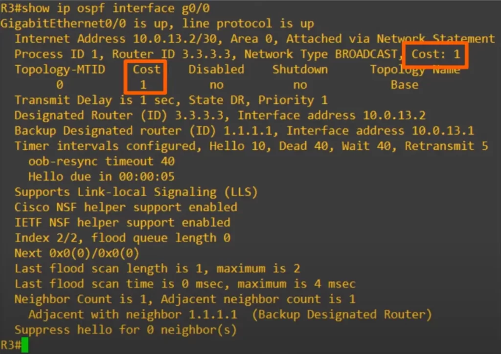
The default OSPF cost on R3’s G0/0 interface is also 1.
A default OSPF cost of 1 on a router’s interface is considered not ideal because it does not allow OSPF to distinguish between different link speeds. This means that all links with a bandwidth of 100 Mbps or more will have the same cost, regardless of whether they are 100 Mbps, 1 Gbps, or 10 Gbps. This can lead to suboptimal routing decisions, as OSPF will not be able to choose the fastest path to a destination.
You can manually configure the OSPF cost for each interface. This will allow you to assign a higher cost to a slower link, so that OSPF will always choose the faster link.
Changing the reference bandwidth
You can change the OSPF cost by using the auto-cost reference-bandwidth command. This command allows you to specify a reference bandwidth for OSPF. The reference bandwidth is used to calculate the cost of an interface.
Here’s the command to change the reference bandwidth from OSPF configuration mode:
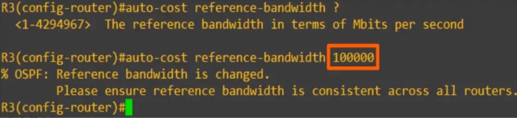
R3(config-router)#auto-cost reference-bandwidth, followed by the numerical value in mbps of the reference bandwidth
Let’s use the command to configure 100,000 as the reference bandwidth.
OSPF cost = reference bandwidth / interface bandwidth, so,
100,000/100 = cost of 1000 for FastEthernet interface
(FastEthernet operates at a speed of 100 mbps)
100,000/1000 = cost of 100 for GigE interface
(Gigabit Ethernet operates at a speed of 1 Gbps or 1000 mbps)
*You should configure a reference bandwidth greater than the fastest links in the network to allow for future upgrades. The 100,000 mbps we configured as the reference bandwidth is equal to a 100 Gbps interface, a 100 times faster than the fastest interfaces in the network, regular Gigabit Ethernet.
The auto-cost reference-bandwidth command is a global configuration command, which means that it applies to all interfaces on the router. If you want to configure a different cost for a specific interface, you can use the ip ospf cost command.
Notice the message displayed in the above CLI output when we configured the reference bandwidth: “Please ensure reference bandwidth is consistent across all routers.” You should configure the same reference bandwidth on all OSPF routers in the network to provide a consistent cost for each interface bandwidth across the network.
OSPF’s metric (cost) cont.
We have set the same OSPF reference bandwidth of 100 Gigabits per second on all of the routers, as we did for R3 above using the auto-cost reference-bandwidth command.
*The OSPF cost to a destination is the total cost of the outgoing or exit interfaces. This is just like Spanning Tree cost. For example, R1’s cost to reach 192.168.4.0/24 is 300. To reach 192.168.4.0/24, a packet would exit R1’s G0/0, R2’s G1/0, and R4’s G1/0. That’s 100 (R1 G0/0) + 100 (R2 G1/0) + 100 (R4 G1/0) = 300 total cost.
We will check R1’s routing table shortly.
*Loopback interfaces have a cost of 1. So what is R1’s cost to reach 2.2.2.2, which is R2’s loopback0 interface?
To reach 2.2.2.2, the packet must exit R1’s G0/0 and R2’s loopback0. The packet does not actually exit any physical interface to reach the virtual loopback interface, but the cost of 1 is added to the metric. So, R1’s cost to reach 2.2.2.2 is 101, i.e.,
100 (R1 G0/0) + 1 (R2 Lo) = 101
Here is R1’s routing table before changing the reference bandwidth of 100 mbps on all the routers.
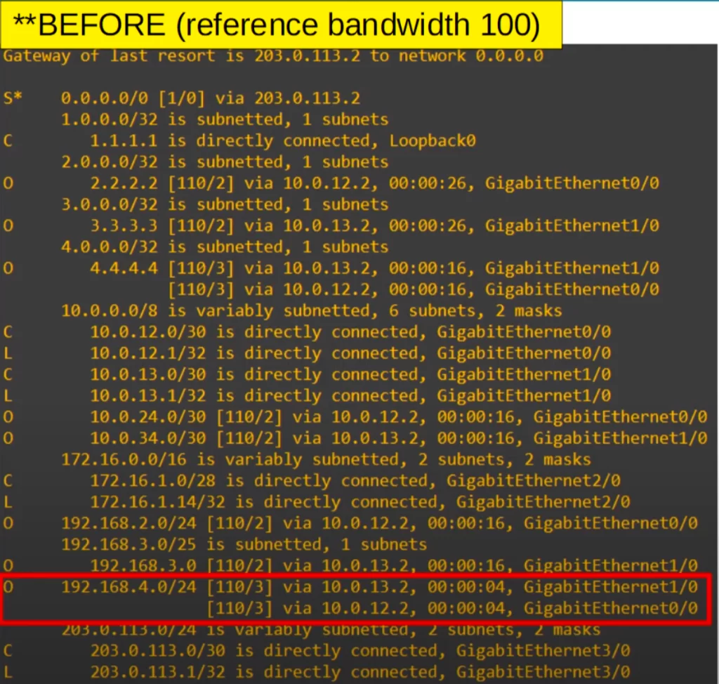
Notice that R1 has two routes to 192.168.4.0/24, one via R2 (10.0.12.2) and one via R3 (10.0.13.2). Even though the connection between R3 and R4 is a slower FastEthernet connection, it has the same cost of 1 as the Gigabit Ethernet interfaces. The default administrative distance for OSPF routes is 110.
Let’s go over the first entry in the red rectangle in the above CLI output:
192.168.4.0/24 [110/3] via 10.0.13.2, 00:00:04, GigabitEthernet1/0
Meaning, there is a route to 192.168.4.0/24 via next hop 10.0.13.2 via R1’s g1/0 with administrative distance/total cost of 110/3. This route was last updated 4 seconds ago .
The total cost is 3 because for the packet to reach 192.168.4.0/24 it will exit three interfaces each with a cost of 1, i.e., R1’s g1/0, R3’s f2/0, and R4’s g1/0. This means all the routers have a reference bandwidth of 100 mbps, as explained earlier.
And here is R1’s routing table after changing the reference bandwidth of each router to 100,000 mbps.
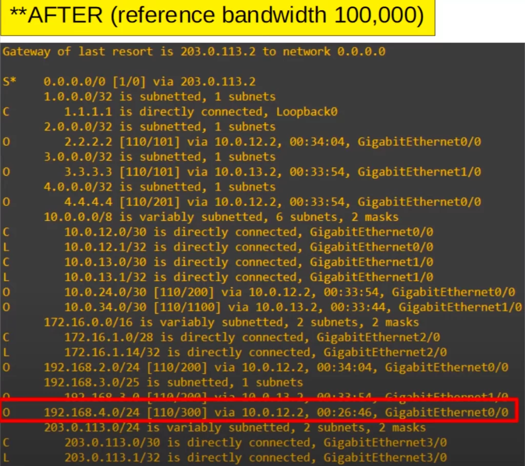
R1 now only adds one route to 192.168.4.0/24 in the routing table, via next hop 10.0.12.2, and the cost is 300 as we calculated. Notice the cost to 2.2.2.2 is 101, also as we calculated.
*A second option to modify the OSPF cost is to manually configure the OSPF cost of an interface.
The ip ospf cost command is used in interface configuration mode to configure the OSPF cost for a specific interface. The cost value can be between 1 and 65535, with a lower value indicating a lower cost.
Use the command ip ospf cost, followed by the cost you want to configure.
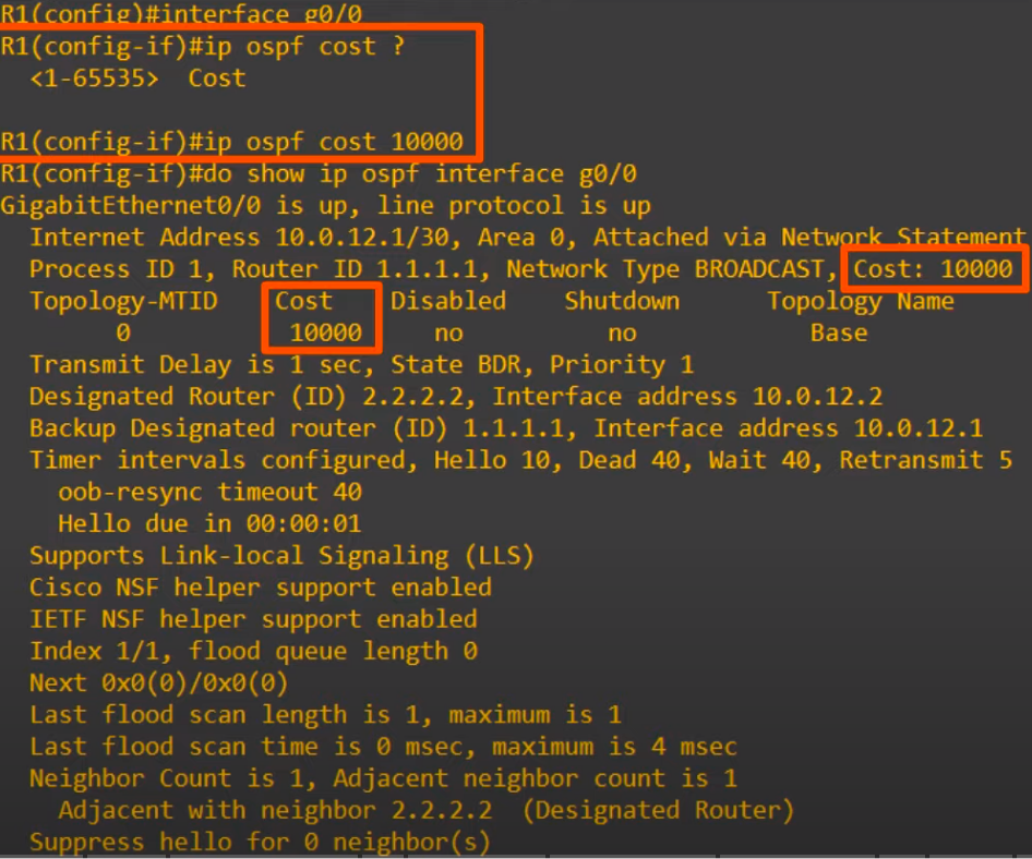
The configured OSPF cost will take priority over the auto-calculated cost. For example, after configuring the cost of R1’s G0/0 interface as 10,000, now you can see the cost is 10,000 instead of 100.
*A third option to change the OSPF cost of an interface is to change the bandwidth of the interface with the bandwidth command. But it is not recommended that you use this method.
Although the bandwidth matches the interface speed by default, changing the interface bandwidth does not actually change the speed at which the interface operates.
If you change the bandwidth of a Gigabit Ethernet interface to 100 mbps, it will still operate at 1 Gigabit per second. However, for the purpose of OSPF’s cost calculation, the bandwidth of 100 mbps will be used. To change the speed at which the interface sends data, use the speed command.
The bandwidth value is used in other calculations, not just the OSPF cost. So it is not recommended to change this value to alter the interface’s OSPF cost. It is recommended that you change the reference bandwidth, and then use the ip ospf cost command to change the cost of individual interfaces if you want.
To change the bandwidth of the interface, use the command bandwidth, followed by the bandwidth in kilobits per second.
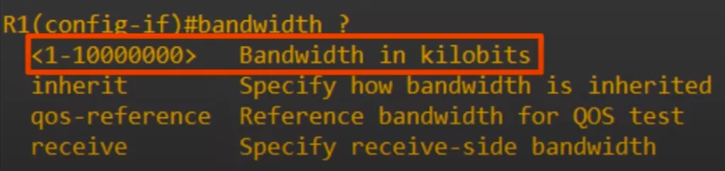
Note, before entering a command like this, you can use the question mark to check the units the command is entered in. For example, in commands involving time, some are entered in seconds, some are entered in minutes. For commands involving speed, some are entered in kilobits, some are entered in megabits.
OSPF cost summary
Let’s summarize the three ways to modify the OSPF cost.
First, to change the reference bandwidth, the command is auto-cost reference-bandwidth and then the reference bandwidth in mbps, entered in OSPF config mode.
R1(config-router)#auto-cost reference-bandwidth mbps
Second, to manually configure the OSPF cost of the interface, the command entered in interface config mode is:
R1(config-if)#ip ospf cost cost
Third, you can change the interface bandwidth, although this is not recommended.
R1(config-if)#bandwidth kbps
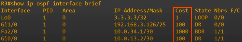
Beside the show ip ospf interface command, there is a quicker way to check the OSPF cost of each interface. The show ip ospf interface brief command gives a convenient overview of each OSPF-enabled interface on the router.
Understand Open Shortest Path First (OSPF) – Design Guide / OSPF cost (cisco.com)
OSPF neighbors
OSPF is implemented in networks to make sure that routers successfully become OSPF neighbors. You can also say, OSPF is implemented in networks to make sure that routers successfully become OSPF adjacencies. It depends on how you want to think about this.
Note: this 15 minute YouTube video by Kevin Wallace Training, LLC will help clarify many key concepts related to OSPF operations: Networking Basics – OSPF Theory
There is a difference between adjacency and neighborship in OSPF.
- Neighborship is a loose relationship between two OSPF routers that are able to communicate with each other. This relationship is established when the routers exchange Hello packets and agree on common OSPF parameters, such as the hello interval and dead interval.
- Adjacency is a more tightly coupled relationship between two OSPF routers that allows them to exchange routing information. This relationship is established when the routers exchange Link State Advertisements (LSAs) and synchronize their link-state databases.
Neighbors are routers on the same network link (segment), sharing the same subnet. These routers exchange hello messages using the multicast address 224.0.0.5 (for IPv4).
Routers first become neighbors and then form OSPF adjacency. Routers in adjacencies do not just exchange hellos, they also exchange LSAs, information to build a link state database (LSDB).
OSPF routers in adjacencies share a common view of the network. They share a common map, an LSDB, that covers an OSPF area. The SPF algorithm is performed on each area.
OSPF routers exchange hello messages to ensure that OSPF routers can discover each other, maintain adjacency with OSPF neighbors, and detect dead neighbors. This helps to keep the OSPF routing table up-to-date and ensures that traffic is routed over the most efficient paths.
OSPF hello messages are sent at a regular interval (by default, 10 seconds on an Ethernet connection and for point-to-point networks, and 30 seconds for broadcast or non-broadcast multi-access networks). When a router receives a hello message from another router, it checks the following information:
- The router ID of the neighbor router.
- The hello interval of the neighbor router.
- The network mask of the interface on which the hello message was received.
If the router ID, hello interval, and network mask match, the routers become OSPF neighbors.
If a router does not receive a hello message from a neighbor router within a certain period of time (by default, 40 seconds for Ethernet connections and point-to-point networks, and 120 seconds for broadcast or non-broadcast multi-access networks), the router assumes that the neighbor router is dead. The router then removes the neighbor router from its OSPF neighbor table and updates its routing table accordingly.
Some additional details about OSPF hello messages:
- The hello message is sent to the multicast address 224.0.0.5. This means that all OSPF routers on the same subnet will receive the hello message.
- The hello message contains a variety of information, including the router ID, hello interval, and network mask.
- The hello message is encrypted if OSPF is configured to use encryption.
RIP hello messages are multicast to the IP address 224.0.0.9. EIGRP hello messages are multicast to the IP address 224.0.0.10.
All OSPF messages are encapsulated in an IP header. The protocol field of the IP header has a value of 89 to indicate OSPF.
OSPF neighbor states (7 states)
For OSPF routers to become neighbors/adjacencies they have to go through various neighbor states. Remember the order and purpose of each state.
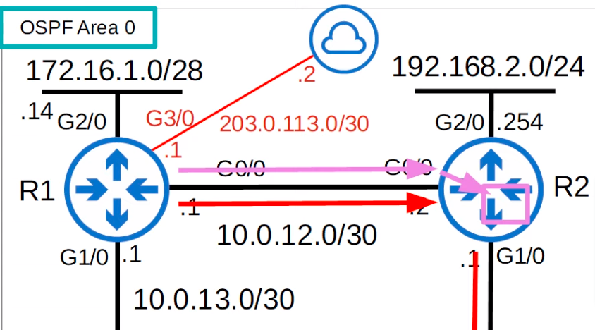
OSPF is activated on R1’s G0/0 interface and R2’s G0/0 interface (see the following diagram).
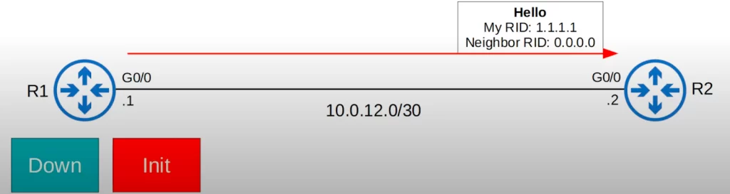
1. OSPF neighbors – down state
In the first OSPF neighbor state, the down state, the two routers send hello packets to the multicast address 224.0.0.5. This is the all OSPF routers multicast address. This means that all OSPF routers on the same subnet will receive the hello packets.
R1’s G0/0 interface fires off an OSPF hello message to 224.0.0.5. Two important fields in the hello message are R1’s router ID (RID) and the neighbor’s router ID. The latter field is still empty since at this state R1 does not know yet about R2.
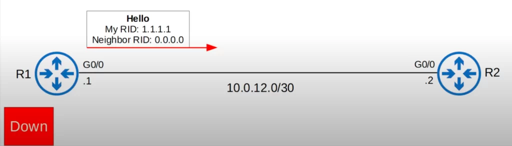
R1 does not know about any OSPF neighbors yet, so the current neighbor state is “down”.
2. OSPF neighbors – init state
When R2 receives the hello packet, it will add an entry for R1 to its OSPF neighbor table. In R2’s neighbor table, the relationship with R1 is now in the init state.
R1 still does not know about R2, so R1 will have no entries in its OSPF neighbor table.
The init state means that R2 received the hello packet, but R2’s own router ID is not in the hello packet. R2’s router ID is 2.2.2.2, but the neighbor router ID in R1’s hello packet is 0.0.0.0.
3. OSPF neighbors – 2-way state
R2 will send a hello packet containing the RID of both routers.
R1 will insert R2 into its OSPF neighbor table.
Then, R1 will send another hello message, this time containing R2’s RID. Now both routers are in the 2-way state.
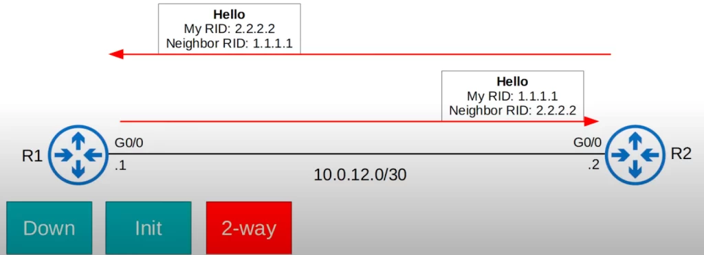
If both routers reach the 2-way state, it means that the conditions to become OSPF neighbors have been met. They are now ready to share LSAs to build a common LSDB.
At this point, the routers are OSPF neighbors. Over the next few neighbor states the routers will share LSAs and form a full OSPF adjacency.
So in the 2-way state, the routers exchange more hello packets, but R1’s router ID is included in R2’s hellos, and R2’s router ID is included in R1’s hellos.
In some network types, a DR (Designated Router) and BDR (Backup Designated Router) will be elected at this point.
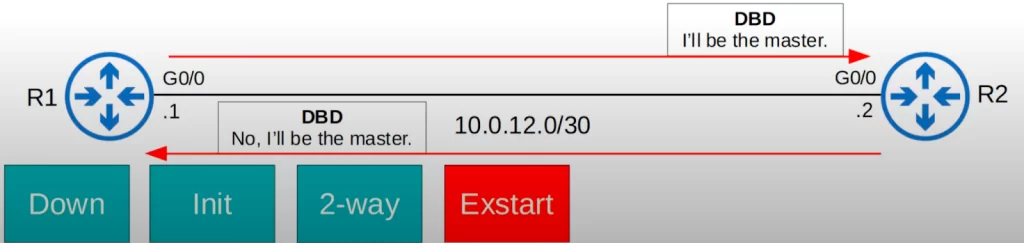
4. OSPF neighbors – exstart state
After the 2-way state, the two routers prepare to exchange information about their LSDB.
But first, the two routers have to choose which router will start the exchange. In the exstart state the two routers decide which router will be the master router and which router will be the slave router. The router with the higher RID will become the master and initiate the exchange. The router with the lower RID will become the slave.
So in this case R2 will be the master and R1 will be the slave.
This master/slave relationship is only needed for this initial exchange of LSDB information.
To decide the master and slave, the two routers exchange DBD (Database Description) packets. DBD packets are also important in the next state. Basically, the purpose of the exstart state is to prepare for the next state.
R1 sends a DBD packet claiming to be the master. However R2 corrects R1. R2 has the higher RID, and says that it will be the master.
5. OSPF neighbors – exchange state
In the exchange state, the routers exchange DBDs which contain a list of the LSAs in their LSDB. These DBDs do not include detailed information about the LSAs, just basic information about what LSAs the neighbor router has.
The routers compare the information in the DBD they received to the information in their own LSDB to determine which LSAs they must receive from their neighbor.
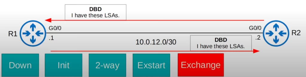
After exchanging DBDs, the routers move to the next state, the Loading state.
6. OSPF neighbors – loading state
In the loading state, routers send each other Link State Request (LSR) messages to request any missing LSAs to make sure each router has the same LSAs.
Then the LSAs are sent in Link State Update (LSU) messages. R2 sends R1 the requested LSAs in an LSU.
Here is an illustration of one side of the exchange. R2 will also send R1 LSRs for any missing LSAs, and R1 will reply to R2 with LSUs.
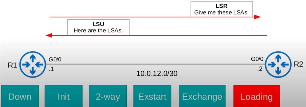
The routers send LSAck messages, another kind of OSPF message, to acknowledge receipt of the LSAs. Now the loading state is complete and the routers have the same LSDB.
7. OSPF neighbors – full state
In the full state, the final OSPF state, the routers have a full OSPF adjacency and identical LSDBs.
The routers continue to send and listen for hello packets to maintain the neighbor adjacency. Another timer called the Dead timer is also used to maintain the neighbor adjacency. Every time a hello packet is received, the Dead timer is reset. If the Dead timer counts down to 0 and no hello message is received, the neighbor is removed. If the neighbors remain up, the routers will continue to share LSAs as the network changes. This ensures that each router has a complete and accurate map of the network (LSDB).
How routers become OSPF neighbors (summary)
First, the connection between R1 and R2 comes up, or OSPF is activated on the interfaces, which starts the process.
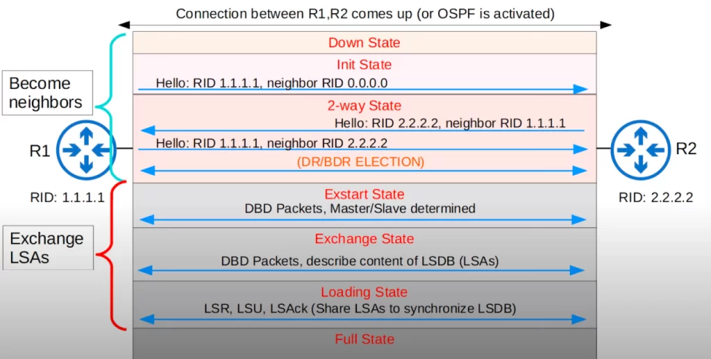
In OSPF there are three main steps in the process of sharing LSAs and determining the best routes to each destination:
1) become neighbors with other routers connected to the same segment,
2) exchange LSAs with neighbor routers, and
3) calculate the best routes to each destination, and insert them into the routing table.
Looking at the process of becoming neighbors again: the first three states (down, init, and 2-way) involve becoming neighbors, and the following three states (exstart, exchange, and loading) involve exchanging LSAs to synchronize the LSDB. And then the routers use the OSPF metric to calculate the best route to each destination.
OSPF message types chart
Here is a summary chart of the 5 different OSPF message types. Notice that they are numbered from 1 to 5, 1 being hello, 2 being DBD, etc.
| Type | Name | Purpose |
| 1 | Hello | Neighbor discovery and maintenance. |
| 2 | Database Description (DBD) | Summary of the LSDB of the router. Used to check if the LSDB of each router is the same. |
| 3 | Link-State Request (LSR) | Requests specific LSAs from the neighbor. |
| 4 | Link-State Update (LSU) | Sends specific LSAs to the neighbor. |
| 5 | Link-State Acknowledgement (LSAck) | Used to acknowledge that the router received a message. |
OSPF show commands
Having covered several OSPF concepts, some of the OSPF show commands should make more sense now. Here is our single area OSPF network again.
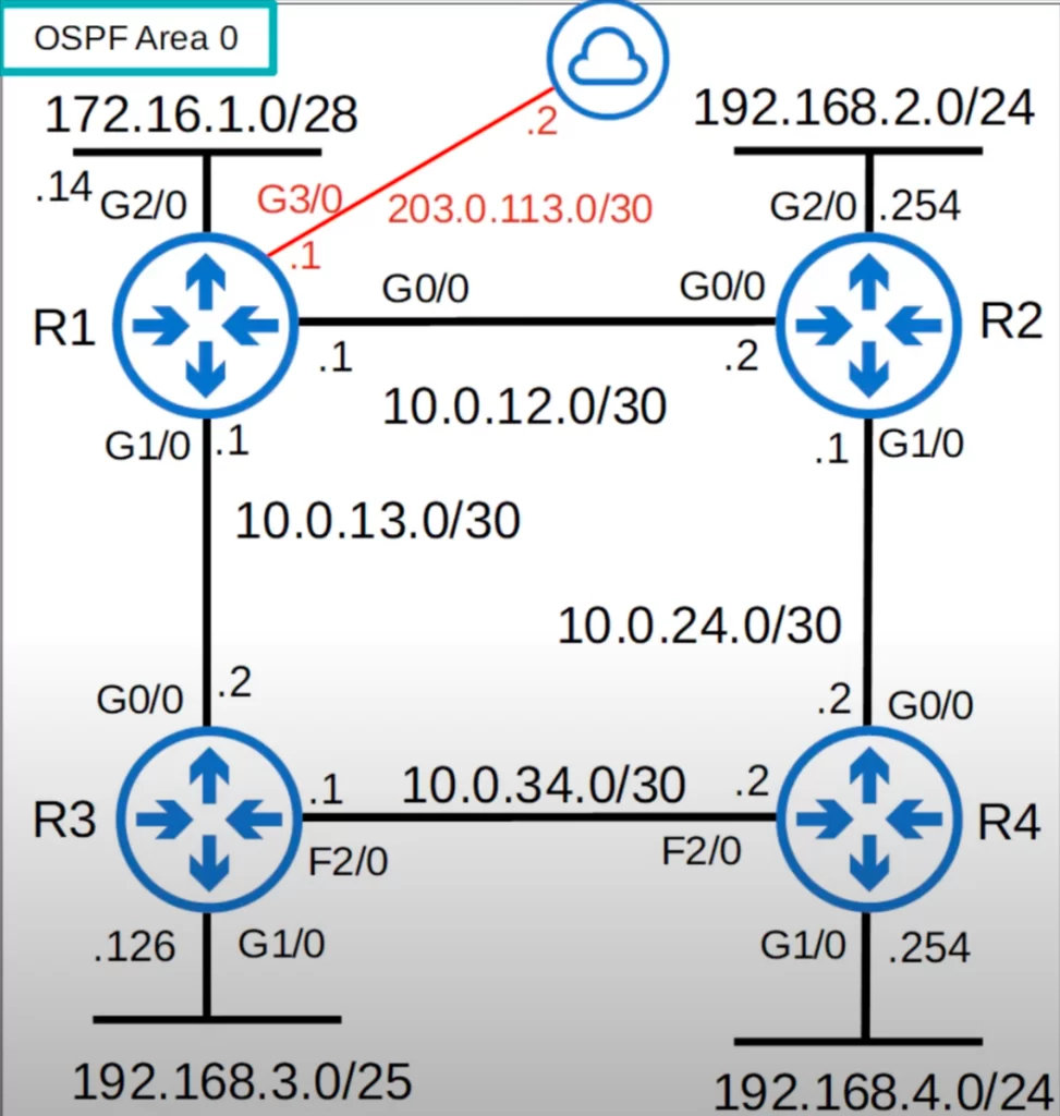
Here is show ip ospf neighbor, entered on R1. Note R1’s full state with both neighbors R3 and R2. Also, both R3 and R2 are Designated Routers (more on DRs in OSPF Part 3).
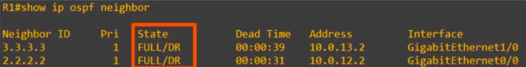
Also notice the Dead time. This counts down from 40, but resets as soon as R1 receives a hello packet from the neighbor. So normally, assuming a hello packet is received every 10 seconds, the timer will count down to 30, reset to 40, count down to 30, reset to 40, etc.
Let’s take another look at show ip ospf interface, looking at R1’s G0/0 interface. You can see the default hello and Dead timers of 10 and 40.
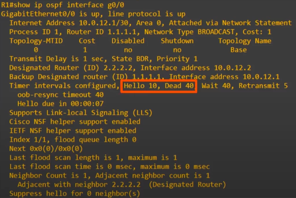
“Hello due in 00:00:07” means that R1 will send a hello message out of the G0/0 interface in 7 seconds. R1 sends a hello message once every 10 seconds.
“Neighbor Count is 1, Adjacent neighbor count is 1” refers to the fact that R1 has only 1 neighbor connected to its G0/0 interface, that’s R2.
“Adjacent with neighbor 2.2.2.2 (Designated Router)” refers to the fact that, as we saw in the above show ip ospf neighbor, R2 is a designated router (DR).
OSPF configurations cont.
Let’s look at a couple of additional configurations.
Recall, the network command in RIP, EIGRP, and OSPF tells the router which interfaces to activate the routing protocol on.
You can enable OSPF directly on an interface, without using the network command. To illustrate, let’s assume that R1 has no OSPF configurations on it yet. Here’s how to enable OSPF on the interfaces.
You can use the following command from interface configuration mode to activate OSPF directly on an interface:
R1(config-if)#ip ospf process-id area area
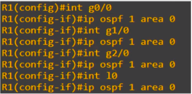
Now OSPF is enabled on those interfaces and we have not even entered OSPF configuration mode.
Next, let’s look at another method to configure passive interfaces.
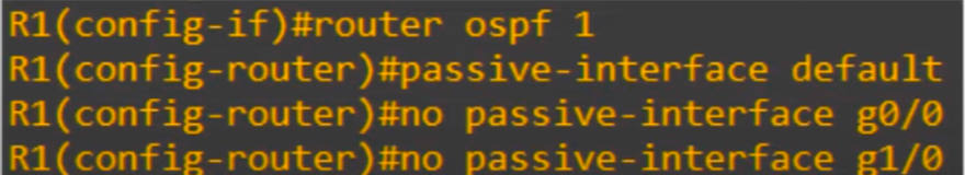
You can configure all the router’s interfaces to be OSPF passive interfaces by default with the command passive-interface default. Then, you can use the command no passive-interface to make only specific interfaces active after.
Configure all interfaces as OSPF passive interfaces:
R1(config)#router ospf 1
R1(config-router)#passive-interface default
Then configure specific interfaces as active:
R1(config-router)#no passive-interface interface-id
Depending on the number of passive interfaces you need to configure, this method might be faster.
If you configure OSPF directly on the interfaces, you will see slightly different output from show ip protocols. The Routing for Networks section is empty.
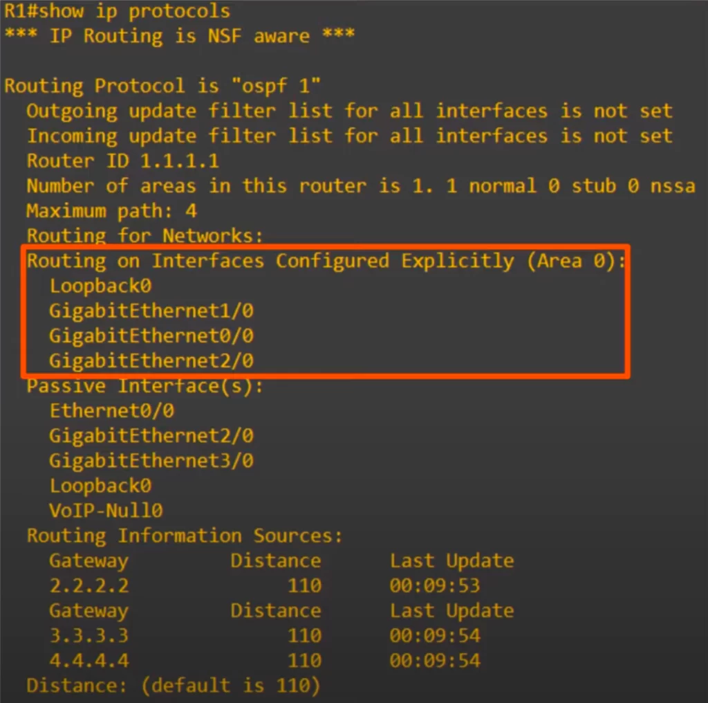
Instead, the interfaces you activated OSPF on are displayed under “Routing on Interfaces Configured Explicitly” (in the red rectangle in the above diagram). The rest of the output is the same.
Command review
>Modify the OSPF cost:
R(config-router)#auto-cost reference-bandwidth mbps
→to change the reference bandwidth of 100 Mbps from OSPF config mode
R(config-if)#ip ospf cost cost
→to manually configure an OSPF cost on a specific interface
R(config-if)#bandwidth kbps
→to change the interface bandwidth
>OSPF show commands:
R#show ip ospf interface [interface | brief]
→to check the ospf cost of an interface
R#show ip ospf neighbor
→to check adjacencies; neighbor ID, priority, adjacency state (FULL/DR, 2way/DROTHER, etc.), Dead time, and neighbor address and interface
>Enable ospf directly on a router interface:
R(config-if)#ip ospf process-id area area
Example:
R1(config)#int g0/0
R1(config-if)#ip ospf 1 area 0
R(config-router)#passive-interface default
→to configure all the router’s interfaces to be OSPF passive interfaces by default
R(config-router)#no passive-interface interface-id
→to configure specific interfaces as active
Free CCNA | Configuring OSPF (2) | Day 27 Lab – Notes
Key learnings
*By default, OSPF’s metric, cost, is automatically calculated by dividing the reference bandwidth by the actual bandwidth of the interface.
Cost = reference bandwidth / interface bandwidth (values less than 1 are converted to 1)
The default reference bandwidth is 100 mbps, so any bandwidth value (speed) equal to or faster than 100 megabits per second has a cost of 1.
*A route’s metric is the total cost of the outgoing interfaces in the route.
*Three methods to change the OSPF cost: auto-cost reference-bandwidth (ospf config mode), ip ospf cost (interface config mode), and bandwidth (interface config mode).
Verifications via show ip ospf interface (privileged EXEC mode), show ip ospf interface brief (privileged EXEC mode), and show ip ospf neighbor (privileged EXEC mode).
>You can modify the reference bandwidth with the auto-cost reference-bandwidth command:
R(config-router)#auto-cost reference-bandwidth mbps
>You can manually configure the cost of an interface with the ip ospf cost command:
R(config-if)#ip ospf cost cost
>One more option to modify an interface’s cost is to modify the interface bandwidth with the bandwidth command, although this isn’t the recommended method.
R(config-if)#bandwidth kbps
*How routers become OSPF neighbors.
*OSPF neighbor states.
*Neighbor vs adjacency.
*Configure OSPF directly on an interface using ip ospf process-id area (global config mode).
How to configure OSPF directly on an interface:
R(config-if)#ip ospf process-id area area-id
*Configure passive OSPF interfaces using passive-interface default +no passive-interface interface-id (interface config mode).
How to configure passive interfaces using the passive-interface default command:
R(config-router)#passive-interface default
Practice quiz questions
Quiz question 1
Put the OSPF neighbor states in the correct order, from 1 to 7.
Down, Init, Two-way, Exstart, Exchange, Loading, and Full.
Here is a mnemonic: Do I Tweet Every Evening Less Friday?
You can find four more practice questions for this lesson (plus a bonus one) in Jeremy’s video lesson OSPF Part 2, cited below.
Key references
Note: The resources cited below (in the “Key references” section of this document) are the main source of knowledge for these study notes/this lesson, unless stated otherwise.
Free CCNA | OSPF Part 2 | Day 27 | CCNA 200-301 Complete Course
Free CCNA | Configuring OSPF (2) | Day 27 Lab | CCNA 200-301 Complete Course
Related content
Compliance frameworks and industry standards
How data flow through the Internet
How to break into information security
IT career paths – everything you need to know
Job roles in IT and cybersecurity
Network security risk mitigation best practices
The GRC approach to managing cybersecurity
The penetration testing process
The Security Operations Center (SOC) career path
Back to DTI Courses